the Creative Commons Attribution 4.0 License.
the Creative Commons Attribution 4.0 License.
 | 11 May 2022
Effectively using multifidelity optimization for wind turbine design
Pietro Bortolotti
Daniel Zalkind
Garrett Barter
Wind turbines are complex multidisciplinary systems that are challenging to design because of the tightly coupled interactions between different subsystems. Computational modeling attempts to resolve these couplings so we can efficiently explore new wind turbine systems early in the design process. Low-fidelity models are computationally efficient but make assumptions and simplifications that limit the accuracy of design studies, whereas high-fidelity models capture more of the actual physics but with increased computational cost. This paper details the use of multifidelity methods for optimizing wind turbine designs by using information from both low- and high-fidelity models to find an optimal solution at reduced cost. Specifically, a trust-region approach is used with a novel corrective function built from a nonlinear surrogate model. We find that for a diverse set of design problems – with examples given in rotor blade geometry design, wind turbine controller design, and wind power plant layout optimization – the multifidelity method finds the optimal design using 38 %–58 % of the computational cost of the high-fidelity-only optimization. The success of the multifidelity method in disparate applications suggests that it could be more broadly applied to other wind energy or otherwise generic applications.
- Article
(3730 KB) - Full-text XML
- BibTeX
- EndNote


Wind turbines are complex systems, where aerodynamic, structural, acoustic, controls, manufacturing, logistic, and technoeconomic considerations are all design drivers. To design the optimal wind energy system, multidisciplinary design optimization (MDO) approaches help capture the interconnected trade-offs among these disciplines while dramatically reducing the time and cost of design processes compared to sequential single-discipline design approaches. The past two decades have seen the development of a variety of MDO models for wind turbine design, such as Giguere and Selig (2000), Fuglsang and Madsen (1999), Ning et al. (2014), Ashuri et al. (2014), Fischer et al. (2014), Pourrajabian et al. (2016), Ning and Petch (2016), Bortolotti et al. (2016), Barlas et al. (2021), among many others.
Choosing the correct fidelity level of analyses used in the MDO process is a crucial decision for the designer, who must meet the need of reasonable accuracy with tractable computational costs. Although lower-fidelity tools offer the possibility to explore a broad solution space and investigate uncommon design choices thanks to the lower computational costs, they often run the risk of oversimplifying the design problem, which could lead to solutions that in reality might underperform or violate unresolved constraints. In contrast, higher-fidelity models are usually incompatible with numerical optimizations that rely on hundreds or thousands of function evaluations. Higher computational costs can therefore be tolerated only when doing spot checks and potential design changes are small.
During the design process, model fidelity usually increases from low to high as more configuration and sizing choices are finalized. Low-fidelity models are usually applied during the early, conceptual stages of design, when many different options, architectures, goals, constraints, etc. are being considered. Because designing these systems using only high-fidelity tools would lead to impossibly long development cycles caused by the computational expense, designers generally start with low-fidelity tools and increase simulation fidelity as the design cycle progresses. This approach usually works fairly well in practice, but it requires frequent interventions and the expertise of the designers. More importantly, it still runs the risk of leading to suboptimal design solutions when the designs are evaluated using more accurate models.
An alternative pathway consists of adopting formal multifidelity design optimization approaches. These methods capture realistic physical trends while reducing the computational cost compared to optimizing using only high-fidelity methods. For applications where single-fidelity design and model iterations work well, multifidelity approaches simply make the design process more efficient by combining information from the low- and high-fidelity models.
Multifidelity optimization methods have a long history across multiple fields, including applied mathematics (Kennedy and O'Hagan, 2000; Forrester et al., 2007; Peherstorfer et al., 2018), aerospace engineering (Robinson et al., 2008; March and Willcox, 2012), and wind energy. Specifically for wind energy, multifidelity methods have been used for aeroelastic blade design (Maki et al., 2012; McWilliam et al., 2017; Abdallah et al., 2019), wind plant layout optimization (Rahbari et al., 2014; Réthoré et al., 2014), and wake steering uncertainty quantification (Quick et al., 2019).
An important subset of multifidelity optimization methods involves surrogate-based optimization (SBO), which is examined within this paper. In SBO, an approximative or reduced-order model is constructed and optimization is performed in that space instead of directly querying high-fidelity models, as detailed by Forrester and Keane (2009). Koziel and Leifsson (2013) give an overview of SBO providing guidance for how best to implement it, whereas other work has focused on efficient global optimization using surrogates (Jones et al., 1998; Viana et al., 2013). The present work further builds upon these efforts by applying multifidelity optimization methods using nonlinear surrogate models for wind energy design problems.
Delving deeper into the literature on multifidelity optimization within wind energy, Maki et al. (2012) use a series of nested and sequential optimizations along with metamodels to minimize the cost of energy for a given turbine design considering multiple fidelities. Réthoré et al. (2014) introduce TOPFARM, a tool for multifidelity layout optimization of wind farms, and they demonstrate sequential optimizations at increasing levels of fidelity to show how optimal results from one model can speed up the design process for a higher fidelity model. McWilliam et al. (2017) used an approximation model management framework (AMMF) approach to perform multifidelity aerostructural optimization of a wind turbine blade. That work established AMMF as a reasonable tool to enable multifidelity blade design, but it showed that the additional complexity of the AMMF algorithm led to slower overall convergence than high-fidelity-only optimization. This shows that the efficacy of multifidelity methods for wind turbine design is both method and model dependent, and there is room for improvement for developing a method that works more generally without expert intervention.
Building on previous work, questions remain about how to best use multifidelity methods for different wind energy applications. For example, depending on the relative computational cost of the low- and high-fidelity models, different approaches might be more effective. Additionally, the optimization problem size directly impacts how effective certain methods are. We address these questions and examine how multifidelity methods can achieve high-performing designs at lower computational cost.
In this paper, we present best practices for using multifidelity optimization methods for wind energy design applications. We do so by first detailing a trust-region-based multifidelity method with a novel correction function built on top of nonlinear surrogate models. We then formulate and solve three optimization problems: aerodynamic blade design for the IEA 15 MW reference wind turbine; a controls optimization using both linearized and nonlinear state–space models; and a wind power plant layout problem. The problems studied here were selected as they examine different disciplines within the larger wind plant design problem and serve as meaningful representative cases to benchmark the multifidelity optimization method against commonly used single-fidelity methods. All tools and application cases studied here are open source, allowing researchers to compare their methods, applications, and results directly with this paper. By solving disparate optimization problems involving different simulation models, we demonstrate how multifidelity methods can be effectively used for the design of complex wind energy systems.
Section 2 introduces the trust-region multifidelity optimization method we have implemented. Then Sect. 3 compares the computational cost and design performance of the multifidelity optimization method as compared to both low- and high-fidelity optimization. Sections 3.1, 3.2, and 3.3 examine case studies concerning aerodynamic blade design, controller design, and power plant layout, respectively. Each case study section details the design problem, approach, and tools used, which differ for each study. Lastly, Sect. 4 presents key findings and takeaways, including which problem types within wind energy are best suited for multifidelity optimization.
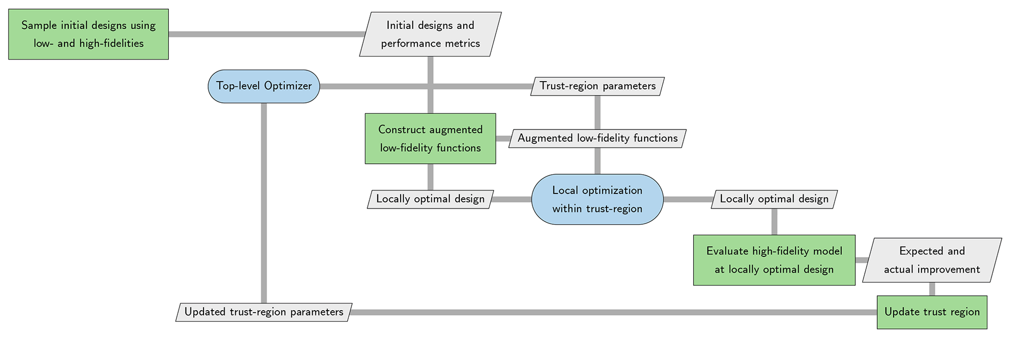
Figure 1XDSM diagram of the trust-region method, specifically showing the top-level and inner-level optimizations.
2.1 Multifidelity methods
In an optimization problem, we seek the minimum of a function within a design space subject to arbitrary constraints. The optimizer selects design variable values, evaluates computational models at that design point to obtain objective and constraint values, and then repeats until convergence is reached. In multifidelity optimization, multiple different types of computational models are queried and information from each model is combined to determine where to sample the design space next. A comprehensive survey of multifidelity methods is presented by Peherstorfer et al. (2018), where various approaches are categorized as one of adaption, fusion, or filtering, with guidelines for matching methods to application. In this work, we focus on the multifidelity optimization method using the adaptation model management strategy and simplified physics-based low-fidelity models. We selected this model management strategy because it is nonintrusive and straightforward to implement in a general manner.
Here we loosely define fidelity as a qualitative measure of the accuracy of the underlying physical equations being modeled compared to the real world. Related to fidelity is the concept of resolution, or how finely discretized a domain or set of inputs might be.
2.2 Trust-region optimization method
We use a trust-region approach to perform multifidelity optimization. This method is well studied in the fields of applied mathematics, computational sciences, and aerospace engineering (Alexandrov et al., 1998, 2001; March and Willcox, 2012). It has also been used in other wind energy research, though those studies focused on different applications (Park and Law, 2015; Yu et al., 2018) or used simplified corrective functions (McWilliam et al., 2017).
The trust-region method used in this work is shown in Algorithm 1 and is adapted from March and Willcox (2012). The method has been modified to relax the mathematical requirements for linearity on the corrective function, which allows for a better representation of nonlinear representations between fidelities. Additionally, constraint values are handled in the same way as the objective function. Specifically, individual surrogate models are created for each function of interest.
Algorithm 1An updated multifidelity trust-region algorithm adapted from March and Willcox (2012).
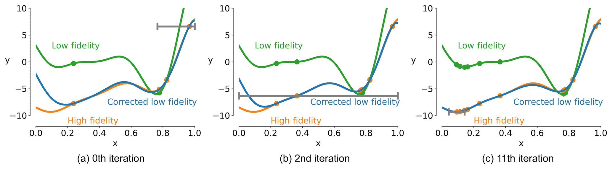
Figure 2Trust-region optimization progression in the 1D example. In the 0th iteration (a), the initial trust region does not contain the entire design space. In the 2nd iteration (b), the trust region has grown as the local optimizer found the best answer at the bounds of the trust region. In the 11th iteration (c), the trust region narrows around the local minima.
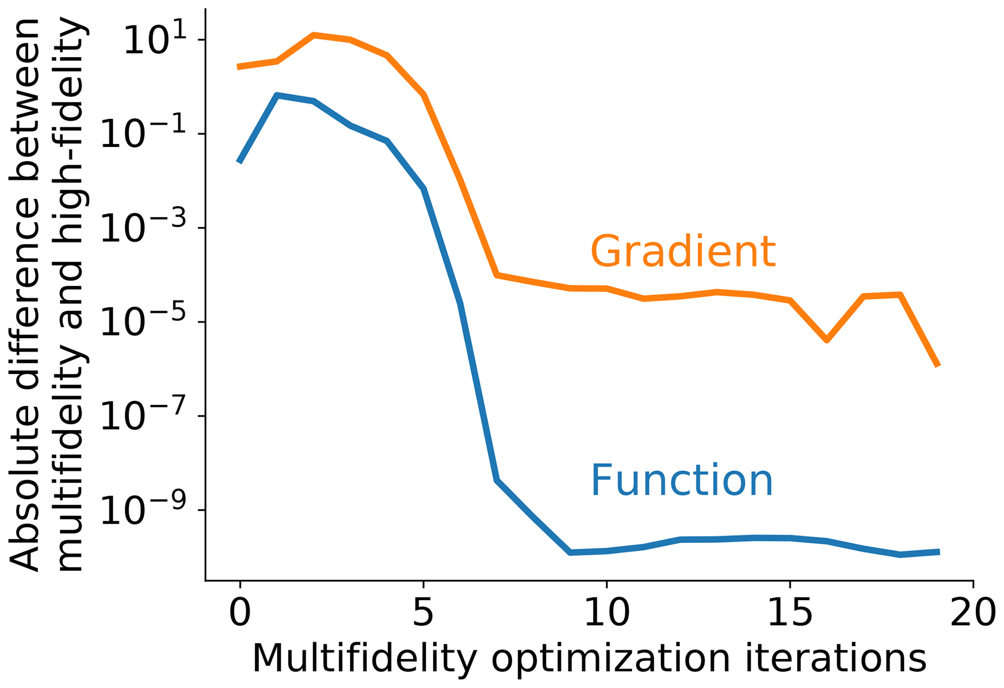
Figure 3Both the function and gradient values of the multifidelity approximation converge to the high-fidelity values for the 1D example.
The trust-region method progression is shown in Fig. 1 using the extended design structure matrix (XDSM) graphical data flow format from Lambe and Martins (2012). The XDSM diagram format shows analysis and optimization processes as on-diagonal blocks in green and blue, respectively. Off-diagonal gray boxes show which data is passed between those process blocks and they are connected by gray lines to show data flow. Following this diagram for the trust-region method, the low- and high-fidelity models are first called at a set of initial design points to establish the corrective function between the fidelities. The corrected function is defined as . Then, a subset of the design space is established where the corrected low-fidelity model is trusted. Local optimization within this region is then performed, and the high-fidelity model is queried at the locally optimal point. Based on the actual reduction in the objective value compared to the expected reduction, the trust region is either expanded or contracted. The local optimization is then repeated within this new trust region, and the process is repeated.
A simple 1D example of how the trust region converges is shown in Fig. 2, which highlights how the corrected low-fidelity model is used to approximate the high-fidelity model. The trust region for local optimization is shown with a gray bar. Based on the criteria defined in step 4 of Algorithm 1, the trust region expands if the newly queried high-fidelity point does not decrease optimality by the expected amount and contracts if the value decrease threshold is met. We also show how the function and gradient values of the multifidelity approximation converge to the high-fidelity values for the same 1D example in Fig. 3.
2.3 Corrective function between low- and high-fidelity models
Within the trust-region method, we need to construct an approximation for the high-fidelity model using the low-fidelity model and a corrective function. This approximation is devised to be interpolative, which means that the corrected low-fidelity model is equal to the high-fidelity model at the points where we have high-fidelity data. This condition is not strictly necessary but leads to better-posed multifidelity problems. In previous work in wind energy (McWilliam et al., 2017), this corrective function was simply an additive and/or multiplicative factor, leading to a first-order linear correlation between the models. When dealing with nonlinear design spaces, it makes sense to use a more complex corrective function that can account for nonlinear differences between the fidelity levels because there is no assurance that the trust region is small enough to support a linear approximation of the high-fidelity space.
In this work, we use a nonlinear surrogate model to construct the corrective function as , which allows us to capture arbitrary correlations between the models. This nonlinear surrogate formulation is especially useful when we do not have an a priori simple understanding of the correlation between the different fidelity levels, which is common in physics-based modeling. Recent advances in surrogate modeling have increased the accuracy for a given model when using a fixed number of data points while simultaneously decreasing computational cost. One example is the Kriging partial least squares (KPLS) method (Bouhlel et al., 2016), which is based on the Kriging method (Cressie, 1988). Typically, as problem dimensionality increases, the cost of training the surrogate model increases as well; however, KPLS has much lower initialization and training costs than ordinary Kriging due to its internal dimension reduction, leading to a lower computational cost when training the model (Bouhlel et al., 2016). Additionally, the gain in surrogate accuracy is generally worth the increased cost compared to using a simple piecewise linear fit.
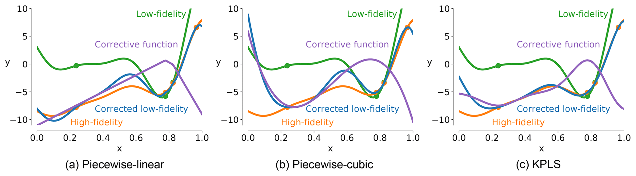
Figure 4Corrective function formulation with piecewise linear reasonably approximating the higher-fidelity model (a), piecewise cubic introducing unwanted oscillations in the approximation (b), and KPLS-based corrective function matching the high-fidelity most accurately (c).
A detailed explanation of KPLS is provided by Bouhlel et al. (2016), including how training cost varies with dimensionality and number of training points. Across multiple benchmarks presented in that paper, KPLS obtains better accuracy in less central processing unit (CPU) time than Kriging. The cost of training the surrogate increases sublinearly as both dimensionality and number of training points increase. These gains are afforded by the partial least squares method that projects the relationships between the output and input variables into a new space formed by the principal components (Bouhlel et al., 2016). The number of high-fidelity function evaluations needed to obtain reasonable accuracy is problem dependent and largely based on the nonlinearity of the design space.
Figure 4 shows the impact of the corrective function on the corrected low-fidelity model for a canonical 1D problem and relatively few data points. Here, we plot the low-fidelity, high-fidelity, corrected low-fidelity, and corrective function all on the same plots. Each case was trained using the same number and location of model samples. Figure 4a shows that using a simple piecewise linear fit achieves reasonable results, but it does not capture the high-fidelity function well. Sensibly, increasing the order of the corrective function might produce a better result, but Fig. 4b shows that a piecewise cubic fit leads to a worse fit, far from the data points. Lastly, Fig. 4c shows how a KPLS-based corrective function does very well at capturing the high-fidelity model trends in between the data points.
Although the trends shown in these figures suggest that KPLS is the best corrective function, the performance and accuracy of these corrections is entirely problem dependent. For other problems, a different surrogate model may be more advantageous. That said, these advanced surrogate modeling techniques generally capture multidimensional nonlinear correlations much better than more simplistic functions, especially when using a small number of high-fidelity data points. Additionally, if we wanted to obtain a better fit with the high-fidelity model, we could use gradient information at each data point to ensure that the corrected low-fidelity model has the same gradient values at those points. For this work, however, we purposefully do not assume that we have any high-fidelity gradient information, which makes the methods presented here applicable to a wider range of real-world tools and applications. For the following case studies, we use a KPLS-based corrective function with the number of sampling points depending on the application. The KPLS implementation is taken from the open-source surrogate modeling toolbox (SMT) presented by Bouhlel et al. (2019) and available at github.com/SMTorg/smt.
Regarding our selected surrogate model as the corrective function, we must note that the multifidelity optimum may not necessarily exactly match the high-fidelity optimum. Whereas prior work focused on producing a provably convergent trust-region approach as detailed by March and Willcox (2012), we do not impose that requirement in this work. This allows for more freedom in the type of corrective function used and is predicated on the basis that the multifidelity optimum is close to the high-fidelity optimum in an engineering sense instead of a numerical one. The following case studies show differences between the optimal results in some cases and are commented on in more detail within their respective sections.
We now study the efficacy of the multifidelity trust-region method on three different case studies representing common optimization problems within wind energy. In order, we examine aerodynamic blade design, controller design, and power plant layout design. Within each subsection, we first detail the computational models used, the optimization problem formulation, and then show the multifidelity method's results. We also perform single-fidelity optimizations using each of the low- and high-fidelity models to have a basis of comparison for the multifidelity results. These single-fidelity optimizations are formulated with the same design variables, constraints, and objectives as in the multifidelity approach. In each case, the single-fidelity optimizations are solved using the gradient-based SNOPT (Sparse Nonlinear OPTimizer, Stanford Business Software, Inc) method (Gill et al., 2005) with finite differencing used to obtain the gradients.
The three case studies show problems with 7, 1, and 14 design variables. This is intended to showcase the multifidelity method's scaling across optimization problems of different sizes. We use the KPLS surrogate as our correction method, which scales well as the problem dimensionality increases (Bouhlel et al., 2016), though the dimensionality of problems we can reasonably solve is limited by the finite-differencing process used to obtain the gradients. The effects of these methods on the case study results are discussed in detail below.
3.1 Blade design optimization
This case study focuses on creating an aerodynamically optimal blade, a common and challenging problem in wind turbine design. Blades are commonly designed using relatively low-fidelity aerodynamic models, such as steady-state blade-element momentum theory (BEMT), which does not capture the effects that unsteady 3D flows have on blade performance. Using multifidelity optimization methods for blade design would allow for more accurate aerodynamic considerations earlier in the design cycle.
3.1.1 Model descriptions and tools used
The multifidelity optimization method is implemented in the Wind Energy with Integrated Servo-control (WEIS) framework (NREL, 2021c). WEIS is a new design tool that enables multifidelity wind turbine design by integrating the capabilities of multiple tools from the National Renewable Energy Laboratory (NREL). Of the numerous WEIS component models, the ones active in the first two case studies in this paper include the systems engineering framework Wind-Plant Integrated System Design & Engineering Model (WISDEM®) (NREL, 2021d), the aeroservoelastic solver OpenFAST (NREL, 2021b), the auto-tuning Reference OpenSource Controller (ROSCO) (NREL, 2020), the wind solver TurbSim (Jonkman, 2009), as well as several pre- and post-processing routines. The primary goal of WEIS is to provide a framework for the controller codesign of floating wind turbines alongside turbine and platform geometry at multiple fidelity levels. In this paper, we do not include floating dynamics, because incorporating that degree of complexity into the other case studies is the focus of future work. The next subsections present more details on the models of WEIS adopted in this work and the formulation of the optimization problem.
Within WEIS, users have the option to individually activate WISDEM and OpenFAST, with additional customization available for all of the various submodules. In this way, numerous simulation pathways are available, creating a spectrum of fidelity options.
WISDEM is built using OpenMDAO (Gray et al., 2019), the open-source Python-based optimization framework developed at the National Aeronautics and Space Administration's Glenn Research Center. WISDEM models the wind turbine as an assembly of blocks, where each block models a specific component of the machine. The blocks are ordered following the load path – namely from the blades toward the tower – and once the machine is sized, cost models are called to compute the levelized cost of energy. WISDEM computes only steady-state performance and loads and is therefore considered a lower-fidelity simulation tool.
Wind turbine aerodynamics in WISDEM are computed with the CCBlade module, which implements the formulation of the BEMT presented in Ning (2014), with hub and tip losses accounted for. The RotorSE module in WISDEM combines the CCBlade-computed aerodynamic loads with a 1D element beam solver, based on Frame3DD (Gavin, 2014), which accounts for centrifugal stiffening but otherwise assumes a rigid rotor with no aeroelastic iteration.
OpenFAST is a multiphysics, multifidelity tool for simulating the coupled dynamic response of wind turbines in the time domain. It is well represented in the literature and has undergone numerous validation studies. In this work, OpenFAST serves as the high-fidelity level of the multifidelity optimization approach.
The aerodynamics in OpenFAST are handled by the module AeroDyn15, whose theory is described in Moriarty and Hansen (2005). AeroDyn15 implements various permutations of the BEMT theory and, since recently, a free-wake vortex aerodynamic model (Shaler et al., 2020). Among the unsteady effects, the airfoil aerodynamics include the Onera stall model. Full aeroelastic coupling is implemented in OpenFAST by combining the aerodynamic loads from AeroDyn with the blade structural dynamics simulated by ElastoDyn using Rayleigh-Ritz shape functions. The user can model the wind as a steady-state flow or via turbulent wind grids with the affiliated TurbSim (Jonkman, 2009) model. OpenFAST also includes two aerodynamic models of the tower – namely the Powles and the Eames models – and couples the turbine elastic behavior with the rotor and tower aerodynamics.
3.1.2 Optimization problem formulation
To study the efficacy of the trust region multifidelity method, we set up a simple blade design optimization case study using the IEA 15 MW reference wind turbine (Gaertner et al., 2020) as the baseline. This reference turbine has a rotor diameter of 242.2 m and a hub height of 150 m. The objective of the study is to maximize the electrical power of the generator at a given wind speed, 9 m s−1, by varying the blade twist and chord. Notably, the problem focuses only on rotor aerodynamic performance and does not consider any structural constraints or subsystem design constraints. For the low-fidelity model, we use the steady-state BEMT solver CCBlade, as described in Sect. 3.1.1. For the high-fidelity model, we use the unsteady BEMT solver within AeroDyn15 with the dynamic generator torque controller active. The inflow includes turbulence, and flapwise and edgewise blade flexibility is accounted for.
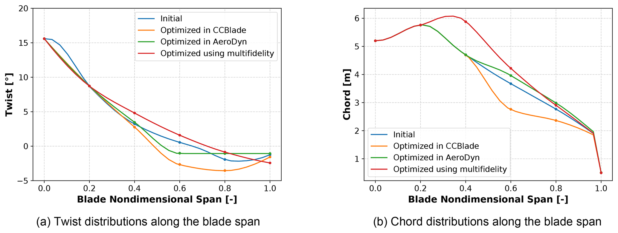
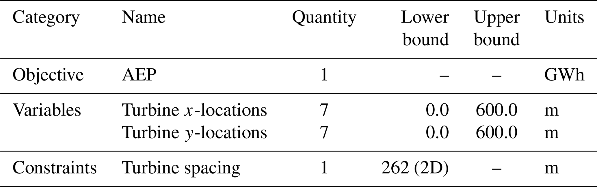
Table 1Optimization problem formulation for the unconstrained power maximization case.

The blade and twist profiles along the blade are controlled by continuous spline interpolations. Each profile is independently parameterized using six control points, with the first two points fixed for both twist and chord and the outermost point fixed for chord. The twist control point design variables act as an adder on top of the original distribution, and the chord control point design variables act as a multiplier. This results in seven design variables, as shown in Table 1.
To fairly evaluate the performance of the multifidelity method, we conducted three different blade chord and twist design optimizations:
-
design optimization using only the low-fidelity model, CCBlade;
-
design optimization using only the high-fidelity model, AeroDyn15;
-
design optimization using the trust-region multifidelity method with the KPLS corrective function.
As a last step, we cross-checked the designs by computing the performance for each of the three blade shapes in both CCBlade and AeroDyn15.
3.1.3 Optimization results
The results of the single-fidelity and multifidelity optimizations are reported in Table 2. The optimization of the chord and twist in CCBlade achieves the highest power of the three designs when evaluated by CCBlade, but the lowest of the three in AeroDyn15. On the contrary, the single-fidelity optimization in AeroDyn15 and the multifidelity optimization successfully identify the configuration generating the highest power in the high-fidelity model, with only small numerical differences in performance between them. This result is even more compelling when considering the computational cost of the three optimizations. The low-fidelity-only optimization completed in just under 9 CPU hours with 360 calls to CCBlade. The high-fidelity-only optimization took nearly three times as long, with more than 1511 function calls to AeroDyn15 due to the noisy gradients that are common in unsteady turbulent simulations. In contrast, the multifidelity optimization made only 63 calls to AeroDyn15 but over 2500 calls to CCBlade, with a net CPU time of 10.61 h, only 19 % higher than the low-fidelity-only optimization.
Table 2Optimal results for aerodynamic blade power maximization.
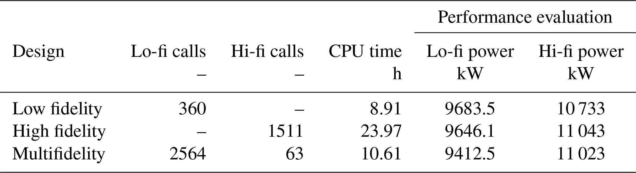
Figure 5 shows the design solutions identified in the three optimizations. The single-fidelity optimization with CCBlade increases the power generation by simultaneously decreasing the twist and chord, effectively increasing the angles of attack along the blade span and narrowing the margin to stall. Both the single-fidelity optimization in AeroDyn15 and the multifidelity optimization choose instead the opposite route and increase the chord and twist, effectively reducing the angles of attack along the blade span. The different design trends can be explained by the unsteadiness of the operational angles of attack at high fidelity caused by the turbulent wind. Such oscillations are less problematic with a higher twist and lower angles of attack, whereas when the blade operates at a lower twist and higher angles of attack, the turbulent wind frequently pushes the blade close to or into stall, increasing drag and decreasing power.
Although the multi- and high-fidelity optimal objective values are close, within 0.2 % of each other, the optimal designs differ greatly. This is because the power-maximization problem results in a quite flat design space where multiple different designs produce close to the same objective value. Given more constraints, a more complex set of design variables, or a different objective function, the flatness and multimodality of the design space would change. For this case study, the low- and high-fidelity models have differently shaped design spaces with different optima. Additionally, because the high-fidelity optimum was obtained using a gradient-based method, the optimal answer is closer to the initial design point. We see that the trust-region multifidelity approach searches the design space more to find its optimal answer.
In this case study, the optimal low- and high-fidelity designs differ due to the models capturing different physics. The rotor design space is relatively flat, as discussed in McWilliam et al. (2021), though adding additional realistic constraints and design variables alters the design space to be better posed, as discussed in Bortolotti et al. (2020). The blade design case study presented showcases the multifidelity method well, by focusing more on the different optimization results than the underlying physical models.
3.2 Controls optimization
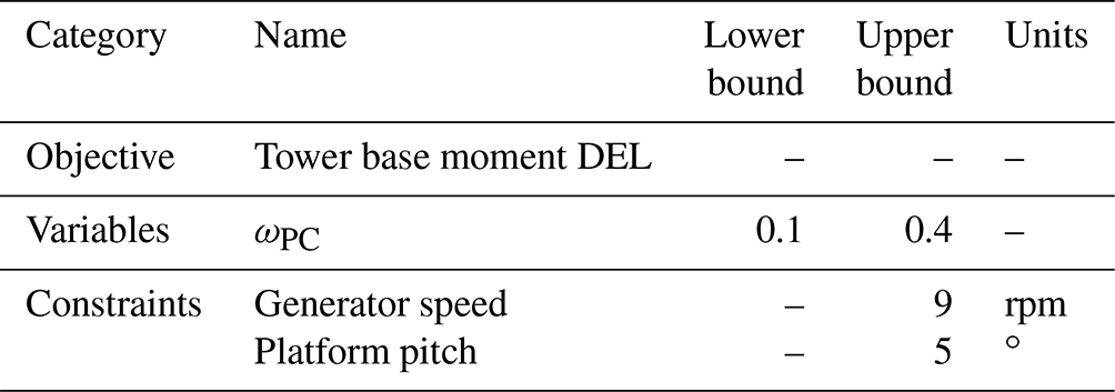
Optimal turbine control, or specifically, determining how to vary the pitch and yaw of the turbine for optimal performance and longevity, is a complex and commonly studied field. To demonstrate multifidelity optimization on a wind turbine control problem, we tune the control bandwidth, ωPC, of the above-rated pitch controller to minimize tower fatigue loads with a constraint on the maximum generator speed. When the generator speed exceeds some limit, the supervisory controller triggers a shutdown procedure, which reduces the net annual energy production (AEP). Tower loads drive the tower design and its capital expenditures. The pitch control bandwidth determines the proportional-integral (PI) gains of the blade pitch controller. Generally, lower bandwidths reduce tower loads but increase generator speed transients, so we expect the results of this optimization procedure to seek the lowest bandwidth, such that the generator speed constraint is not violated.
3.2.1 Model descriptions and tools used
We simulate both a linearized and nonlinear version of the IEA 15 MW wind turbine with the University of Maine's VolturnUS semisubmersible (Allen et al., 2020) in extreme turbulence with a mean wind speed of 16 m s−1. For the nonlinear simulation, we use OpenFAST with the ROSCO controller (NREL, 2020) and a full-field turbulent wind input generated using TurbSim. When this turbulent wind input is sampled by the blades, it results in 3P (per revolution) oscillating loads on the tower. The nonlinear OpenFAST model is run for 800 simulation seconds, which requires approximately 3 min on a standard laptop computer, and represents the high-fidelity model for this case study.

Figure 6High- and low-fidelity control models. The high-fidelity model runs OpenFAST with the ROSCO controller and a full-field (FF) turbulent wind input. The low-fidelity models are described in Eqs. (1)–(3) and use a rotor-averaged wind speed as the input. Both models output time series that can be processed to derive operational and load measures.
To serve as the low-fidelity model, we simulate a linearized turbine and control model, which requires less than 3 s on a standard laptop computer. To create these low-fidelity models, we run OpenFAST in its linear mode, which creates linearized snapshots of the turbine at several azimuth positions for a fixed wind speed (Jonkman and Jonkman, 2016). These linear snapshots are averaged using the multiblade coordinate transform (Bir, 2010) to create a linear time-invariant system relative to the turbine's operating points:
where u, x, and y are the inputs, states, and outputs of the linearized turbine, respectively. The input and output operating points, uop and yop, respectively, and the state-space matrices A, B, C, and D are determined during the OpenFAST linearization process. When multiple wind speeds, uh, are linearized, we construct a set of state-space systems, which can be interpolated based on the mean wind speed, uh, so the system matrices and operating points are a function of uh. In this study, we focus on above-rated control, and we linearize the turbine model at mean wind speeds of 14, 16, and 18 m s−1.
For the pitch control input, which is part of u, we connect the output of a linearized ROSCO controller:
where kP and kI are the PI gains of the pitch controller, and s is the floating feedback gain. The PI gains are a function of the bandwidth, ωPC, and turbine parameters (Abbas et al., 2022). Generally, as the design variable ωPC increases, the PI gains also increase.
The inputs to the controller are the generator speed, ωg, and an acceleration measurement from the nacelle inertial measurement unit (IMU) in the nodding direction, ; these are in y. When the linear turbine and control models are connected, we have a set of closed-loop linear turbine models that depend on the wind speed.
Instead of a full-field turbulent wind input, as in the high-fidelity model, the rotor average wind speed is used to simulate the linear model. The mean rotor average wind speed is used to determine the single closed-loop linear model from the set by linearly interpolating the state-space matrices and operating points. We then integrate the linear system over time, which results in a time series that is similar to the nonlinear model (Fig. 7). Nonlinear aerodynamic and hydrodynamic effects are not captured in the linear state-space model, but they are part of the operating points. In the linear simulations, a constant operating point is chosen for the whole 800 s simulation (with the first 200 s typically omitted as startup transients).

Figure 7Comparison between the time histories generated from the nonlinear and linearized OpenFAST simulations. The linearized model generally has a smoother response than the nonlinear simulation.
Both the linear and nonlinear turbine outputs can be processed to compute the generator speed maxima (constraint) and the damage equivalent loading (DELs) on the tower (objective), as shown in Fig. 8. In general, trends, or changes, in the linear and nonlinear models are in agreement and as expected: increasing the pitch control bandwidth increases tower DELs and platform motion, while decreasing generator speed transients. The linear models do not capture the 3P harmonic loading on the tower, which accounts for most of the difference in the tower base fore–aft DELs between the two models. Finally, the magnitude of the optimization constraints (maximum generator speed and platform pitch angle) are more accurately sampled from the nonlinear simulations; therefore, these constraints are active only in the nonlinear simulations, which creates a good stress test for the multifidelity optimization, where some constraints are violated only in the high-fidelity simulation.

Figure 8The linearized and nonlinear functions of interest as we vary the pitch controller bandwidth, ωPC.
3.2.2 Optimization problem formulation
The objective, design variables, and constraints for the controls optimization problems are shown in Table 3.
Table 3Optimization problem formulation for the controls optimization case.
3.2.3 Optimization results
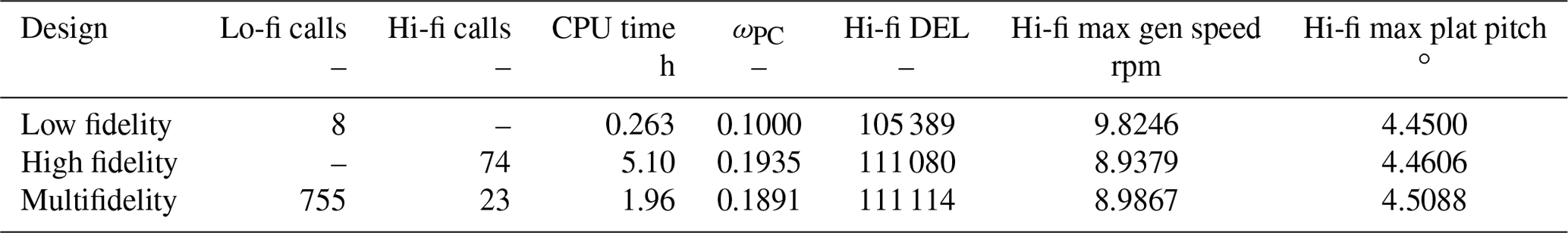
As in the previous case study, we performed single-fidelity optimization using both the low- and high-fidelity models and compared the results to the multifidelity trust-region method. Table 4 contains the optimal ωPC values and the corresponding functions of interest from each optimization. Using the high-fidelity optimization to evaluate true performance, the low-fidelity-only optimization finds an infeasible solution that violates the generator speed constraint. Revisiting Fig. 8, this is expected due to the linearized model not resolving the same magnitude or trends found in the nonlinear model. Although the optimal pitch control bandwidths in the high- and multifidelity optimizations differ, the actual difference in objective value is relatively small, approximately 0.03 %, and the constraints are satisfied in both cases.
Table 4 also shows that the multifidelity method finds an optimal answer using 62 % less computational expense than the high-fidelity optimization. The one-time cost of linearizing the model across three wind speeds is included for both the low- and multifidelity computational cost columns. Specifically, this upfront cost requires 944 core-seconds, but then each function call to the low-fidelity model is quite low, at 0.55 core-seconds. Each function call to the high-fidelity model requires 248 core-seconds.
3.3 Wind power plant layout optimization
Wind power plant layout optimization is the practice of placing wind turbines within a plant to minimize the power production losses caused by wakes from upstream turbines. This is a well studied and challenging optimization problem due to the inherent multimodality of the design space (Samorani, 2013; Baker et al., 2019; Khan and Rehman, 2013; Stanley and Ning, 2019). Turbine–wake interactions require high-fidelity simulations, including large-eddy simulations, to correctly resolve the highly complex flows within a wind power plant (Fleming et al., 2013; Churchfield et al., 2016); however, the large computational expense of these simulations limits their use in design optimization problems, which has encouraged the development of wind power plant simulation tools that straddle multiple levels of fidelity (Sprague et al., 2020; Réthoré et al., 2014). In this case study, we optimize the layout of turbines using multiple different wake models and resolutions to represent different levels of fidelity.
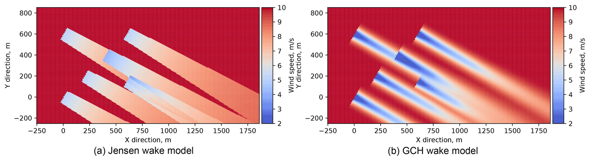
Figure 9Simplistic velocity deficits of the Jensen wake model (Jensen, 1983) (a) versus the more accurately resolved flow field of the GCH model (King et al., 2021) (b).
3.3.1 Model descriptions and tools used
To more easily study how wind turbine layout and controls affect plant performance using less computational cost, multiple analytic wake models have been developed, including the Jensen (Jensen, 1983), Gaussian (Bastankhah and Porté-Agel, 2014), and Gauss–Curl Hybrid (GCH) (King et al., 2021) models. Listed in order of increasing fidelity, these analytic models capture simplified wake physics and have been verified against high-fidelity simulations and validated against experimental results (King et al., 2021).
In this paper, we use the Jensen and GCH as the low- and high-fidelity wake models, respectively. The Jensen wake model uses a simplistic velocity deficit to represent the wake, and this deficit is summed when wakes interact using the sum-of-squares method (Jensen, 1983). Additionally, the velocity deficit fans out linearly behind the turbine. The wakes from the Jensen model for the initial plant used in this study are shown in Fig. 9a. The GCH model modifies the Gaussian model (Bastankhah and Porté-Agel, 2014) by including analytic approximations from the curl model (Martínez-Tossas et al., 2019), which leads to a wake model that better resembles results from high-fidelity simulations. These more complex flow interactions are visible in Fig. 9b, which also uses a sum-of-squares method for wake interaction.
These wake models are already integrated into FLOw Redirection and Induction in Steady State (FLORIS) (NREL, 2021a), a controls-oriented wake-modeling tool that performs wind power plant simulation and optimization. FLORIS is an open-source tool that provides a common application programming interface for multiple wake models, which allows us to easily investigate different levels of fidelity.
In addition to using different wake models, our low- and high-fidelity models for this problem use different wind roses and wind speed bin resolutions, leading to accuracy and computational differences caused by both fidelity and resolution. The low-fidelity model samples six equally spaced wind directions (60∘ bins) and five wind speeds from 0 to 26 m s−1, whereas the high-fidelity model samples 18 wind directions (20∘ bins) and 14 wind speeds from 0 to 26 m s−1. These relatively coarse discretizations were selected so that the optimization studies could be easily run on a laptop workstation. Both models use a Weibull distribution for the wind speed frequencies.
3.3.2 Optimization problem formulation
For this study, we optimize the locations of seven wind turbines within an area of 360 000 m2. Additionally, we impose a two-rotor-diameter (2D or 262 m) spacing constraint between turbines to create a well-posed optimization problem. We aggregate these turbine–turbine spacing constraints using the Kreisselmeier–Steinhauser functional (Poon and Martins, 2007), which reduces the number of constraints from 21 to 1, producing a less complex optimization problem. This problem formulation leads to 14 design variables, one objective, and one constraint, as shown in Table 5. The wind turbine model is based on the NREL 5 MW reference turbine (Jonkman et al., 2009) and is provided within FLORIS.

Figure 10The optimal layout found by the high-fidelity-only optimization (82.368 GWh AEP) (a) and the multifidelity method (81.972 GWh AEP) (b).
Table 5Optimization problem formulation for the wind power plant layout AEP maximization case.
3.3.3 Optimization results
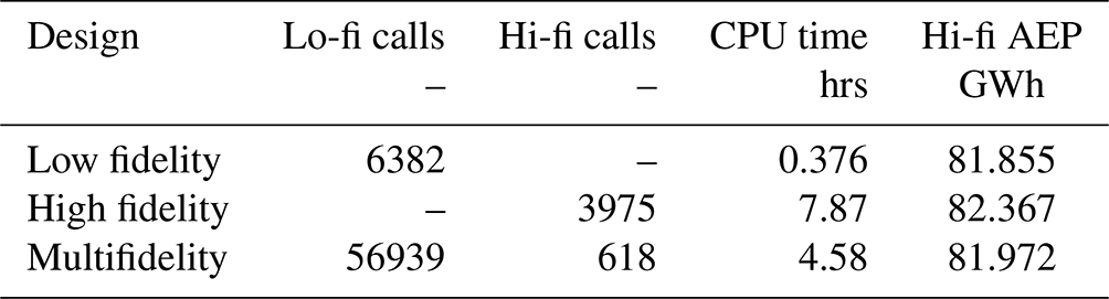
As in the first two case studies, we performed single-fidelity and multifidelity optimizations for this plant layout case, with the high-fidelity AEP evaluated at the optimal design from each method shown in Table 6. Each call to the low- and high-fidelity models took 0.212 and 7.13 s, respectively, meaning that the high-fidelity model is 33.6 times as expensive as the low-fidelity model to evaluate. Overall, we see that the multifidelity method takes 58 % as many core-hours to find an optimal answer as the high-fidelity method. The multifidelity method resulted in a better layout than the low-fidelity optimization; however, this AEP value was less than that from the high-fidelity optimization. Examining the physical layouts from the high- and multifidelity cases shown in Fig. 10, the results do not appear drastically different, although only one wind direction and speed from the wind rose is shown. The main difference between the two cases lies in the location of the central turbine, which is farther north in the high-fidelity case. Note that in all cases, the turbine spacing constraint is not active at the optimal design; thus, the trade-off between the computational savings and the optimality of the obtained design would vary based on the number of wind turbine locations optimized.
Table 6Optimization results for the wind power plant layout AEP maximization case.
This wind power plant layout problem presents an interesting case for the multifidelity method due to the highly nonlinear design space as well as the number of design variables. The corrective function used to correlate the two fidelity levels needs to be able to capture sharp changes in AEP with respect to changes in turbine location. By using surrogate corrective functions, as detailed in Sect. 2.3, we are able to account for the design space nonlinearities. As the number of design variables increases, however, the number of points needed to correctly correlate the two fidelities also increases. This trend is not due to the type of corrective function used but is instead due to the well-known “curse of dimensionality”, which dictates that the cost of constructing an accurate representation of a high-dimensional space increases greatly as the number of dimensions increases. These costs are problem dependent, and this power plant layout problem is known to be highly nonlinear and high dimensional, which leads to a relatively large number of training points to correctly correlate the low- and high-fidelity models.
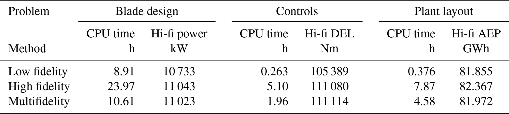
Table 7Each case is summarized here, showing the multifidelity method takes less computational time than the high-fidelity-only optimization while finding improved designs compared to the low-fidelity-only approach.
We have shown that multifidelity optimization methods are effective for a variety of wind energy applications to decrease the computational cost needed to find an optimal design. Optimizing using only a low-fidelity model might miss important physical trends that the high- and multifidelity approaches will correctly capture. Researchers can adopt the multifidelity method described here following the example cases uploaded to the code repository.
Across three distinct applications – aerodynamic blade design, controls tuning, and wind power plant layout optimization – we have shown that obtaining an optimal result requires less computational cost compared to high-fidelity optimization, as depicted in Table 7. In each case, the multifidelity method finds a more optimal result than the low-fidelity-only approach. Due to multimodality in the problems' design spaces and optimization tolerances, the multifidelity method does not necessarily converge to exactly the high-fidelity optimum. We discussed the optimal designs and the differences between the high- and multifidelity results in detail in each of the case study subsections.
Although we used a traditional trust-region approach for multifidelity optimization, we offered a new corrective function technique based on efficient KPLS surrogate models, and we demonstrated its efficacy across three case studies. In this way, the methods and results presented in this paper should be useful to wind energy researchers who seek optimal designs when using multiple levels of model fidelity.
There are some limitations to the types of design problems for which multifidelity methods are effective. Specifically, there needs to be an established model fidelity hierarchy with one model known to be of higher fidelity than another. If the accuracy of the models is unknown, then the trust-region method presented here is ill posed. Each model used in the multifidelity method must receive the same inputs and return the same outputs so the corrective function between fidelity levels can be constructed. Additionally, higher-dimensional design spaces lead to larger computational cost in order to adequately explore the space. This is especially true in the case of multimodal problems where there may be many local optima, such as the plant layout problem. Finally, multifidelity methods are less beneficial when there is not a large difference between the computational expense of the models. Many engineering design problems meet these requirements, but special care is needed to select appropriate levels of model fidelity and to pose a reasonable optimization problem.
Future work could involve more complicated design problems, additional fidelity tiers, or different types of model disciplines. For example, further work could solve the blade aerodynamic design problem using the multifidelity method with BEM and a computational fluid dynamics or vortex wake model. Additionally, performance improvements from other multifidelity methods could be incorporated, such as gradient-based surrogate models using high-fidelity gradients, or more intelligent expected improvement algorithms to find the next point to query using the high-fidelity model. This would decrease the computational cost of performing these optimizations but would require additional developer time to construct the framework and models correctly. As the optimization problems increase in complexity, the best multifidelity strategy might differ, including which type of corrective function or how many correlative design points to use. A series of model fidelities could also be considered, with nested trust regions to conduct the model fidelity management. Lastly, in this paper we examined multiple disciplines in wind energy systems engineering, but there are additional subsets of model disciplines that could benefit from design exploration through these multifidelity methods.
All code and models used in this paper are open source and provided here: https://doi.org/10.5281/zenodo.6109699 (Jasa et al., 2022).
GB, PB, and JJ conceptualized the study. GB performed funding acquisition, project administration, and supervision. JJ developed the methodology and PB, DZ, and JJ performed formal analysis, investigation, and visualization. All authors contributed to original draft preparation and editing.
The contact author has declared that neither they nor their co-authors have any competing interests.
Publisher's note: Copernicus Publications remains neutral with regard to jurisdictional claims in published maps and institutional affiliations.
This work was authored by the National Renewable Energy Laboratory, operated by Alliance for Sustainable Energy, LLC, for the US Department of Energy (DOE) under Contract No. DE-AC36-08GO28308. Funding provided by US Department of Energy Advanced Research Projects Agency – Energy. The views expressed in the article do not necessarily represent the views of the DOE or the US Government. The US Government retains and the publisher, by accepting the article for publication, acknowledges that the US Government retains a nonexclusive, paid-up, irrevocable, worldwide license to publish or reproduce the published form of this work, or allow others to do so, for US Government purposes.
This research was performed using computational resources sponsored by the Department of Energy's Office of Energy Efficiency and Renewable Energy and located at the National Renewable Energy Laboratory.
This research has been supported by the US Department of Energy, Advanced Research Projects Agency – Energy (grant no. DE-AC36-08GO28308).
This paper was edited by Michael Muskulus and reviewed by Michael Muskulus and one anonymous referee.
Abbas, N. J., Zalkind, D. S., Pao, L., and Wright, A.: A reference open-source controller for fixed and floating offshore wind turbines, Wind Energ. Sci., 7, 53–73, https://doi.org/10.5194/wes-7-53-2022, 2022. a
Abdallah, I., Lataniotis, C., and Sudret, B.: Parametric hierarchical kriging for multi-fidelity aero-servo-elastic simulators – Application to extreme loads on wind turbines, Probabil. Eng. Mech., 55, 67–77, 2019. a
Alexandrov, N. M., Dennis, J., Lewis, R. M., and Torczon, V.: A trust-region framework for managing the use of approximation models in optimization, Struct. Optimiz., 15, 16–23, 1998. a
Alexandrov, N. M., Lewis, R. M., Gumbert, C. R., Green, L. L., and Newman, P. A.: Approximation and model management in aerodynamic optimization with variable-fidelity models, J. Aircraft, 38, 1093–1101, 2001. a
Allen, C., Viselli, A., Dagher, H., Goupee, A., Gaertner, E., Abbas, N., Hall, M., and Barter, G.: Definition of the UMaine VolturnUS-S Reference Platform Developed for the IEA Wind 15-Megawatt Offshore Reference Wind Turbine, Tech. Rep. NREL/TP-76773, International Energy Agency, https://doi.org/10.2172/1660012, 2020. a
Ashuri, T., Zaaijer, M. B., Martins, J. R. R. A., van Bussel, G. J. W., and van Kuik, G. A. M.: Multidisciplinary Design Optimization of Offshore Wind Turbines for Minimum Levelized Cost of Energy, Renew. Energy, 68, 893–905, https://doi.org/10.1016/j.renene.2014.02.045, 2014. a
Baker, N. F., Stanley, A. P., Thomas, J. J., Ning, A., and Dykes, K.: Best practices for wake model and optimization algorithm selection in wind farm layout optimization, in: AIAA Scitech 2019 Forum, 7–11 January 2019, San Diego, California, p. 0540, https://doi.org/10.2514/6.2019-0540, 2019. a
Barlas, T., Ramos-García, N., Pirrung, G. R., and González Horcas, S.: Surrogate-based aeroelastic design optimization of tip extensions on a modern 10 MW wind turbine, Wind Energ. Sci., 6, 491–504, https://doi.org/10.5194/wes-6-491-2021, 2021. a
Bastankhah, M. and Porté-Agel, F.: A new analytical model for wind-turbine wakes, Renew. Energy, 70, 116–123, 2014. a, b
Bir, G. S.: User's Guide to MBC3: Multi-Blade Coordinate Transformation Code for 3-Bladed Wind Turbine, Tech. Rep. NREL/TP-500-44327, National Renewable Energy Laboratory, https://www.nrel.gov/docs/fy10osti/44327.pdf (last access: 26 April 2022), 2010. a
Bortolotti, P., Bottasso, C. L., and Croce, A.: Combined preliminary–detailed design of wind turbines, Wind Energ. Sci., 1, 71–88, https://doi.org/10.5194/wes-1-71-2016, 2016. a
Bortolotti, P., Dixon, K., Gaertner, E., Rotondo, M., and Barter, G.: An efficient approach to explore the solution space of a wind turbine rotor design process, J. Phys.: Conf. Ser., 1618, 042016, https://doi.org/10.1088/1742-6596/1618/4/042016, 2020. a
Bouhlel, M. A., Bartoli, N., Otsmane, A., and Morlier, J.: Improving Kriging Surrogates of High-Dimensional Design Models by Partial Least Squares Dimension Reduction, Struct. Multidisciplin. Optimiz., 53, 935–952, https://doi.org/10.1007/s00158-015-1395-9, 2016. a, b, c, d, e
Bouhlel, M. A., Hwang, J. T., Bartoli, N., Lafage, R., Morlier, J., and Martins, J. R. R. A.: A Python surrogate modeling framework with derivatives, Adv. Eng. Softw., 135, 102662, https://doi.org/10.1016/j.advengsoft.2019.03.005, 2019. a
Churchfield, M., Wang, Q., Scholbrock, A., Herges, T., Mikkelsen, T., and Sjöholm, M.: Using high-fidelity computational fluid dynamics to help design a wind turbine wake measurement experiment, J. Phys.: Conf. Ser., 753, 032009, https://doi.org/10.1088/1742-6596/753/3/032009, 2016. a
Cressie, N.: Spatial prediction and ordinary kriging, Math. Geol., 20, 405–421, 1988. a
Fischer, G. R., Kipouros, T., and Savill, A. M.: Multi-objective optimisation of horizontal axis wind turbine structure and energy production using aerofoil and blade properties as design variables, Renew. Energy, 62, 506–515, 2014. a
Fleming, P., Gebraad, P., van Wingerden, J.-W., Lee, S., Churchfield, M., Scholbrock, A., Michalakes, J., Johnson, K., and Moriarty, P.: SOWFA super-controller: A high-fidelity tool for evaluating wind plant control approaches, Tech. rep., NREL – National Renewable Energy Lab., Golden, CO, USA, https://www.nrel.gov/docs/fy13osti/57175.pdf (last access: 26 April 2022), 2013. a
Forrester, A. I. and Keane, A. J.: Recent advances in surrogate-based optimization, Prog. Aerosp. Sci., 45, 50–79, 2009. a
Forrester, A. I., Sóbester, A., and Keane, A. J.: Multi-fidelity optimization via surrogate modelling, P. Roy. Soc. A, 463, 3251–3269, 2007. a
Fuglsang, P. and Madsen, H. A.: Optimization method for wind turbine rotors, J. Wind Eng. Indust. Aerodynam., 80, 191–206, 1999. a
Gaertner, E., Rinker, J., Sethuraman, L., Zahle, F., Anderson, B., Barter, G., Abbas, N., Meng, F., Bortolotti, P., Skrzypinski, W., Scott, G., Feil, R., Bredmose, H., Dykes, K., Sheilds, M., Allen, C., and Viselli, A.: IEA Wind TCP Task 37: Definition of the IEA 15-Megawatt Offshore Reference Wind Turbine, Tech. Rep. NREL/TP-75698, International Energy Agency, https://doi.org/10.2172/1603478, 2020. a
Gavin, H. P.: Frame3DD. Static and Dynamic Structural Analysis of 2D and 3D Frames, version 0.20140514+, http://frame3dd.sourceforge.net/ (last access: 26 April 2022), 2014. a
Giguere, P. and Selig, M.: Blade geometry optimization for the design of wind turbine rotors, in: 2000 ASME Wind Energy Symposium, January 2000, Reno, NV, USA, p. 45, https://doi.org/10.2514/6.2000-45, 2000. a
Gill, P. E., Murray, W., and Saunders, M. A.: SNOPT: An SQP algorithm for large-scale constrained optimization, SIAM Rev., 47, 99–131, 2005. a
Gray, J. S., Hwang, J. T., Martins, J. R. R. A., Moore, K. T., and Naylor, B. A.: OpenMDAO: An open-source framework for multidisciplinary design, analysis, and optimization, Struc. Multidisciplin. Optimiz., 59, 1075–1104, https://doi.org/10.1007/s00158-019-02211-z, 2019. a
Jasa, J., Bortolotti, P., Zalkind, D., and Barter, G.: Data and models for “Effectively using multifidelity optimization for wind turbine design” Zenodo [code], https://doi.org/10.5281/zenodo.6109699, 2022. a
Jensen, N.: A note on wind generator interaction, no. 2411 in Risø-M, Risø National Laboratory, http://citeseerx.ist.psu.edu/viewdoc/download?doi=10.1.1.456.4080&rep=rep1&type=pdf (last access: 26 April 2022), 1983. a, b, c
Jones, D. R., Schonlau, M., and Welch, W. J.: Efficient global optimization of expensive black-box functions, J. Global Optimiz., 13, 455–492, 1998. a
Jonkman, B.: TurbSim User's Guide: Version 1.50, Tech. Rep. NREL/TP-500-46198, National Renewable Energy Laboratory, https://www.nrel.gov/docs/fy09osti/46198.pdf (last access: 26 April 2022), 2009. a, b
Jonkman, J., Butterfield, S., Musial, W., and Scott, G.: Definition of a 5-MW reference wind turbine for offshore system development, Tech. rep., NREL – National Renewable Energy Lab., Golden, CO, USA, https://doi.org/10.2172/947422, 2009. a
Jonkman, J. M. and Jonkman, B. J.: FAST modularization framework for wind turbine simulation: full-system linearization, J. Phys.: Conf. Ser., 753, 082010, https://doi.org/10.1088/1742-6596/753/8/082010, 2016. a
Kennedy, M. C. and O'Hagan, A.: Predicting the output from a complex computer code when fast approximations are available, Biometrika, 87, 1–13, 2000. a
Khan, S. A. and Rehman, S.: Iterative non-deterministic algorithms in on-shore wind farm design: A brief survey, Renew. Sustain. Energ. Rev., 19, 370–384, 2013. a
King, J., Fleming, P., King, R., Martínez-Tossas, L. A., Bay, C. J., Mudafort, R., and Simley, E.: Control-oriented model for secondary effects of wake steering, Wind Energ. Sci., 6, 701–714, https://doi.org/10.5194/wes-6-701-2021, 2021. a, b, c
Koziel, S. and Leifsson, L.: Surrogate-based modeling and optimization, Springer, https://doi.org/10.1007/978-1-4614-7551-4, 2013. a
Lambe, A. B. and Martins, J. R. R. A.: Extensions to the Design Structure Matrix for the Description of Multidisciplinary Design, Analysis, and Optimization Processes, Struct. Multidisciplin. Optimiz., 46, 273–284, https://doi.org/10.1007/s00158-012-0763-y, 2012. a
Maki, K., Sbragio, R., and Vlahopoulos, N.: System design of a wind turbine using a multi-level optimization approach, Renew. Energy, 43, 101–110, 2012. a, b
March, A. and Willcox, K.: Provably convergent multifidelity optimization algorithm not requiring high-fidelity derivatives, AIAA J., 50, 1079–1089, 2012. a, b, c, d, e
Martínez-Tossas, L. A., Annoni, J., Fleming, P. A., and Churchfield, M. J.: The aerodynamics of the curled wake: a simplified model in view of flow control, Wind Energ. Sci., 4, 127–138, https://doi.org/10.5194/wes-4-127-2019, 2019. a
McWilliam, M. K., Zahle, F., Pavese, C., and Blasques, J. P.: Multi-fidelity optimization of horizontal axis wind turbines, in: 35th Wind Energy Symposium, 9–13 January 2017, Grapevine, Texas, p. 1846, https://doi.org/10.2514/6.2017-1846, 2017. a, b, c, d
McWilliam, M. K., Zahle, F., Dykes, K., Bortolotti, P., Ning, A., Gaertner, E., Macquart, T., Merz, K., and Ruiz, A. I.: IEA Wind Energy Task 37-System Engineering-Aerodynamic Optimization Case Study, in: AIAA Scitech 2021 Forum, p. 1412, https://doi.org/10.2514/6.2021-1412, 2021. a
Moriarty, P. J. and Hansen, A.: AeroDyn Theory Manual, Tech. Rep. NREL/TP-500-36881, National Renewable Energy Laboratory, https://www.nrel.gov/docs/fy05osti/36881.pdf (last access: 26 April 2022), 2005. a
Ning, A. and Petch, D.: Integrated design of downwind land-based wind turbines using analytic gradients, Wind Energy, 19, 2137–2152, https://doi.org/10.1002/we.1972, 2016. a
Ning, S. A.: A simple solution method for the blade element momentum equations with guaranteed convergence, Wind Energy, 17, 1327–1345, https://doi.org/10.1002/we.1636, 2014. a
Ning, S. A., Damiani, R., and Moriarty, P. J.: Objectives and constraints for wind turbine optimization, J. Solar Energ. Eng., 136, 041010, https://doi.org/10.1115/1.4027693, 2014. a
NREL: ROSCO, Version 2.1.1, GitHub [code], https://github.com/NREL/rosco (last access: 26 April 2022), 2020. a, b
NREL: FLORIS, Version 2.2.5, GitHub [code], https://github.com/NREL/floris (last access: 26 April 2022), 2021a. a
NREL: OpenFAST, v2.5.0, GitHub [code], https://github.com/OpenFAST/openfast (last access: 26 April 2022), 2021b. a
NREL: WEIS, v1.0, GitHub [code], https://github.com/WISDEM/WEIS (last access: 26 April 2022), 2021c. a
NREL: WISDEM, v3.2.0, GitHub [code], https://github.com/WISDEM/WISDEM (last access: 26 April 2022), 2021d. a
Park, J. and Law, K. H.: A Bayesian optimization approach for wind farm power maximization, in: Smart Sensor Phenomena, Technology, Networks, and Systems Integration 2015, vol. 9436, International Society for Optics and Photonics, p. 943608, https://doi.org/10.1117/12.2084184, 2015. a
Peherstorfer, B., Willcox, K., and Gunzburger, M.: Survey of Multifidelity Methods in Uncertainty Propagation, Inference, and Optimization, SIAM Rev., 60, 550–591, https://doi.org/10.1137/16M1082469, 2018. a, b
Poon, N. M. K. and Martins, J. R. R. A.: An Adaptive Approach to Constraint Aggregation Using Adjoint Sensitivity Analysis, Struct. Multidisciplin. Optimiz., 34, 61–73, https://doi.org/10.1007/s00158-006-0061-7, 2007. a
Pourrajabian, A., Afshar, P. A. N., Ahmadizadeh, M., and Wood, D.: Aero-structural design and optimization of a small wind turbine blade, Renew. Energy, 87, 837–848, 2016. a
Quick, J., Hamlington, P. E., King, R., and Sprague, M. A.: Multifidelity uncertainty quantification with applications in wind turbine aerodynamics, in: AIAA Scitech 2019 Forum, 7–11 January 2019, San Diego, California, p. 0542, https://doi.org/10.2514/6.2019-0542, 2019. a
Rahbari, O., Vafaeipour, M., Fazelpour, F., Feidt, M., and Rosen, M. A.: Towards realistic designs of wind farm layouts: Application of a novel placement selector approach, Energ. Convers. Manage., 81, 242–254, 2014. a
Réthoré, P.-E., Fuglsang, P., Larsen, G. C., Buhl, T., Larsen, T. J., and Madsen, H. A.: TOPFARM: Multi-fidelity optimization of wind farms, Wind Energy, 17, 1797–1816, 2014. a, b, c
Robinson, T. D., Eldred, M. S., Willcox, K. E., and Haimes, R.: Surrogate-Based Optimization Using Multifidelity Models with Variable Parameterization and Corrected Space Mapping, AIAA J., 46, 2814–2822, https://doi.org/10.2514/1.36043, 2008. a
Samorani, M.: The wind farm layout optimization problem, in: Handbook of wind power systems, Springer, 21–38, https://doi.org/10.1007/978-3-642-41080-2_2, 2013. a
Shaler, K., Branlard, E., and Platt, A.: OLAF User’s Guide and Theory Manual, Tech. Rep. NREL/TP-5000-75959, National Renewable Energy Laboratory, https://doi.org/10.2172/1659853, 2020. a
Sprague, M. A., Ananthan, S., Vijayakumar, G., and Robinson, M.: ExaWind: A multifidelity modeling and simulation environment for wind energy, J. Phys.: Conf. Ser., 1452, 012071, https://doi.org/10.1088/1742-6596/1452/1/012071, 2020. a
Stanley, A. P. J. and Ning, A.: Massive simplification of the wind farm layout optimization problem, Wind Energ. Sci., 4, 663–676, https://doi.org/10.5194/wes-4-663-2019, 2019. a
Viana, F. A., Haftka, R. T., and Watson, L. T.: Efficient global optimization algorithm assisted by multiple surrogate techniques, J. Global Optimiz., 56, 669–689, 2013. a
Yu, X., Zhang, W., Zang, H., and Yang, H.: Wind power interval forecasting based on confidence interval optimization, Energies, 11, 3336, https://doi.org/10.3390/en11123336, 2018. a