the Creative Commons Attribution 4.0 License.
the Creative Commons Attribution 4.0 License.
 | 19 Aug 2024
Underestimation of strong wind speeds offshore in ERA5: evidence, discussion and correction
Jorge Garza
Offshore wind power plants have become an important element of the European electrical grid. Studies of metocean site conditions (wind, sea state, currents, water levels) form a key input to the design of these large infrastructure projects. Such studies rely heavily on reanalysis datasets which provide decades-long model time series over large areas. In turn, these time series are used for assessing wind, water levels and wave conditions and are thereby key inputs to design activities such as calculations of fatigue loads and extreme loads and platform elevations. In this article, we address a known deficiency of one these reanalysis datasets, ERA5, namely that it underestimates strong wind speeds offshore. If left uncorrected, this poses a design risk (high and extreme wind, waves and water level conditions are underestimated). Firstly, comparisons are made against CFSR/CFSv2 reanalyses as well as high-quality wind-energy-specific in situ measurements from floating lidar systems. Then, the ERA5 surface drag formulation and its sea state dependency are analysed in detail, the conditions of the bias identified, and a correction method is suggested. The article concludes with proposing practical and simple ways to incorporate publicly available, high-quality wind energy measurement datasets in air–sea interaction studies alongside legacy measurements such as met buoys.
Please read the corrigendum first before continuing.
-
Notice on corrigendum
The requested paper has a corresponding corrigendum published. Please read the corrigendum first before downloading the article.
-
Article
(7350 KB)
-
The requested paper has a corresponding corrigendum published. Please read the corrigendum first before downloading the article.
- Article
(7350 KB) - Full-text XML
- Corrigendum
- BibTeX
- EndNote


Offshore wind power plants help reduce carbon emissions from the power sector. They have gradually evolved from small demonstration projects (Vindeby, commissioned in 1991) to commercial-scale demonstration projects (Horns Reef 1, Nysted) in the early 2000s. Today, they stand as integral components of the European power grid (ENTSO-E, 2024).
Atmospheric boundary layer (ABL) wind datasets from numerical weather prediction modelling systems (NWP models) are routinely used for the purpose of assessing the offshore wind resources and for characterising sea state, water level and current conditions at offshore wind farm locations (NWP models provide inputs to hydrodynamic and spectral wave models). Global reanalysis datasets such as CFSR (Saha et al., 2010), CFSv2 (Saha et al., 2014) and ERA5 (Hersbach et al., 2020) are widely used for these purposes as they are publicly available, are free of charge and cover long periods (decades).
Despite performing among the best (see Ramon et al., 2019, a study considering 77 tall tower sites which concludes that “ERA5 near-surface wind dataset offers the best estimates of mean wind speed and variability at turbine hub heights”), the NWP model used for producing ERA5 suffers from a major drawback for engineering purposes: it underestimates strong wind speeds offshore close to the surface, for instance at 10 m (a nominal elevation often used for hydrodynamic and spectral wave modelling). This is documented for instance in Bentamy et al. (2021), a study which uses in situ far and near offshore measurements; see their Figs. 4 and 5, which display an ERA5 bias for strong wind conditions. Similarly, Alday et al. (2021) refer to Pineau-Guillou et al. (2018) for documenting the ERA5 bias and propose a piece-wise linear correction. The bias is documented in Solbrekke et al. (2021), Spangehl et al. (2023), and Meyer and Gaslikova (2024) as well at measurement locations in the North Sea where ERA5 performs worse than other datasets. Therefore, for engineering applications the ERA5 10 m wind speed values are often corrected to ensure that site conditions design values are not underestimated; see for instance DHI (2023). In effect, for design, slightly conservative values are typically desirable: model results that underestimate high wind speeds, and thereby also large waves, pose a design risk (of loads that are too small as well as platform elevations that are too low). As a result, and despite their shortcomings (differences in land–sea masks and grid resolution, poorer correlation with in situ measurements, no wind speed time series close to a modern turbine hub height), CFSR and CFSv2 remain, in the authors' experience, the preferred datasets for driving engineering hydrodynamic and spectral wave modelling systems.
This ERA5 bias has not been widely discussed in the scientific literature, and it may not be clear to all ERA5 users that the data need to be corrected. Also, the methods published so far only partially address the bias: most often, they correct 10 m winds only and/or use site-specific corrections; see Alday et al. (2021) or DHI (2023). The present article proposes a novel approach to both topics. After having provided elements of wind speed modelling in Sect. 1, we compare ERA5 and CFSv2 model time series at selected locations, with each other and against in situ measurements in Europe and America in Sect. 2. The ERA5 strong wind bias is discussed in Sect. 3: a detailed analysis of the ERA5 drag formulation is provided, and a simple correction method is suggested for wind speeds between 10 and 100 m using analytical ABL wind profile expressions from the literature. The measurement datasets all come from high-quality, publicly available met mast and floating lidar system (FLS) datasets; these are described in Sect. 1.
The main objectives of this article are (1) to present evidence of the ERA5 underestimation of strong wind speeds, (2) discuss the reason for this underestimation and propose a simple corrective method, and (3) argue for using publicly available, high-quality FLS measurements and met mast datasets for air–sea interaction studies, along with legacy measurements such as met buoys. In Sect. 4 and with references to the recent literature, suggestions are made regarding practical actions and research initiatives.
This article provides references to recent works regarding air–sea interaction and drag formulations. Yet, it does not take a scientific stand on the nature of these interactions. Instead, it merely tries to bring a practitioner's perspective to this long-lasting discussion: for design purposes, an accurate depiction of both wind and sea state in reanalysis datasets is required, and useful, quality datasets are readily available for validation work.
1.1 Elements of wind profile modelling
As explained for instance in Peña et al. (2008) and its references such as Stull (1988), in the layer close to the surface where the Monin–Obukhov similarity theory (MOST) is valid, the mean wind speed U at a given elevation z above the surface is given by
where is the friction velocity at the surface, z0 is the roughness length, κ is the von Kármán constant (here taken equal to 0.4), L is the Obukhov length and ψm is an atmospheric stability-dependent function derived from experiments. Above the surface layer, this expression needs to be supplemented with additional terms: the height of the boundary layer zi and a length scale LMBL, which is a characteristic length scale of the eddies in the ABL (see the original in Gryning et al., 2007, and references therein).
Over water, the Charnock relationship is used for linking roughness length and friction velocity (see Peña et al., 2008, and Eq. 3.26 of ECMWF, 2016a):
where αCh and αM are sea-state-dependent parameters and ν is the air kinematic viscosity (term only relevant for very low wind speeds). We use αM=0.11 following Sect. 3.2.4 of ECMWF (2016a). Equations (1) and (2) are widely used in NWP modelling systems such as the Global Forecast System (GFS), the Integrated Forecast System (IFS) and the Weather Research and Forecasting (WRF) Model. The term αCh is referred to as the Charnock parameter and is either kept constant (for instance in Peña et al., 2008, or in CFSR/CFSv2; see Renfrew et al., 2002) or made dependent on sea state conditions. In this article, we focus on the IFS Cy41r2 (ERA5) implementation. See Eq. (3.11) of ECMWF (2016b), where the atmospheric and ocean models are coupled via
where τ is the wind stress (, where ρa is the air density), τw is the wave stress (from the waves to the atmosphere) and is a constant. For all practical purposes, a neutral drag coefficient Cd,n can be derived and is often used for comparing model and measurement results:
where Un is the wind speed for neutral conditions evaluated using Eq. (1) and (negligible buoyancy).
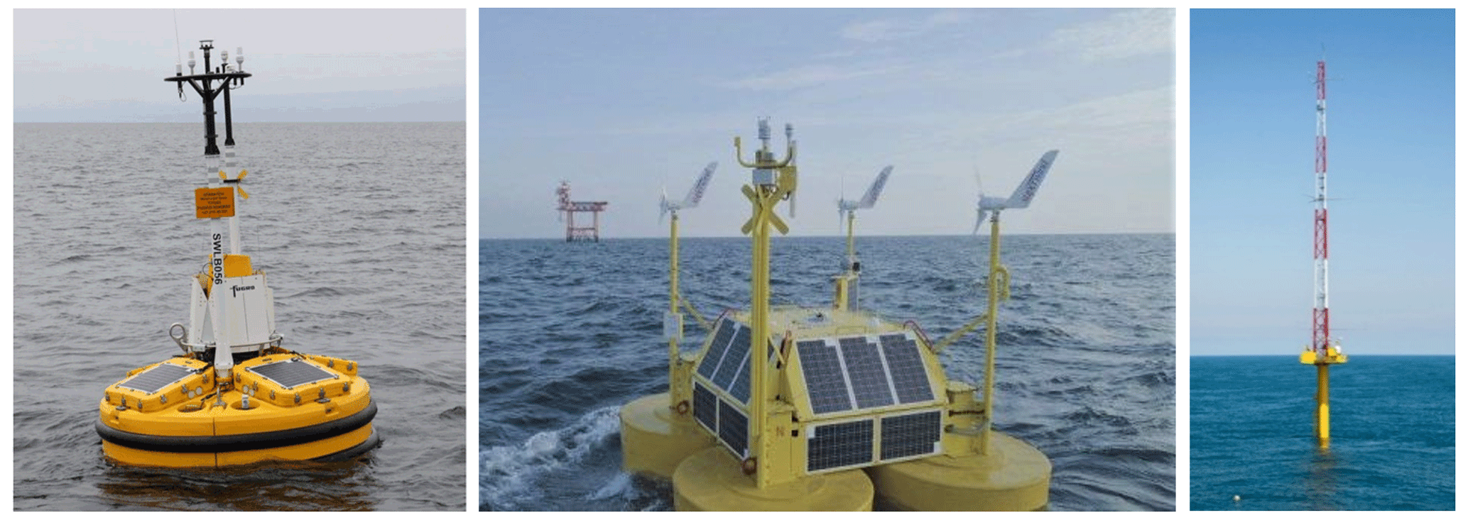
Figure 1Photographs of the floating lidar systems (left panel: Fugro, middle panel: EOLOS) as well as the IJmuiden mast (right panel). Sources: Fugro, EOLOS and Wind op Zee.
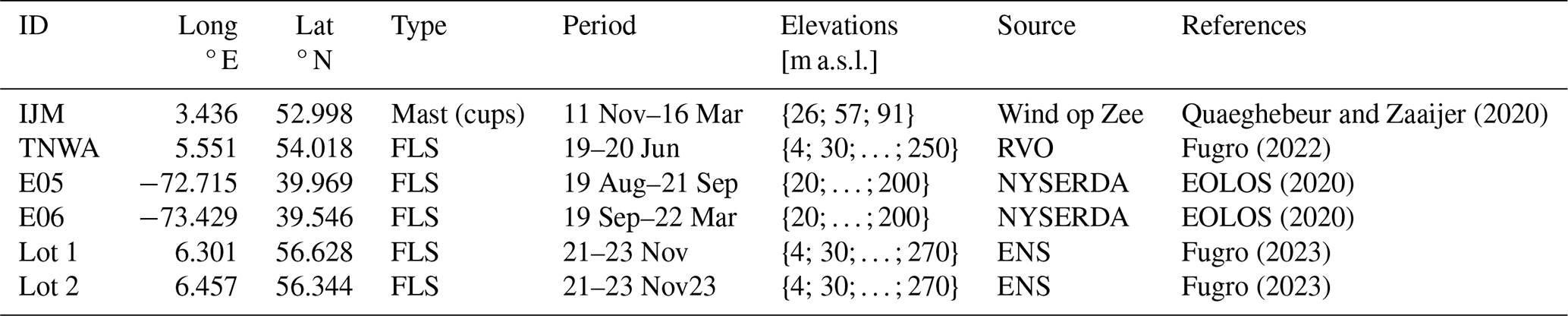
Table 1High-level description of the measurement datasets used in this article. Detailed information can be found in the references provided in the table.
1.2 Measurement data description
In this article, we use well-documented and well-validated, high-quality, publicly available measurement datasets from the wind energy industry such as floating lidar systems and a met mast (cup anemometer); see Fig. 1. Legacy instruments such a met buoys have been left out intentionally due to the poor quality and traceability of these measurements in comparison to the former datasets. A discussion is provided in Sect. 4 on future works and the advantages of adding such wind energy measurements alongside legacy instruments to decrease modelling uncertainty.
The measurements have been chosen from the comprehensive list of datasets available on the Wind Resource Assessment Group wiki page (see https://groups.io/g/wrag/wiki/13236, last access: 11 August 2024). Their locations are marked in red in Fig. 2, and a high-level description is provided in Table 1 (except for M6 and 62001, where no measurement data are used). All measurement locations lie far offshore, where land–sea mask effects are negligible for the wind directional bins selected for the analyses (see Sect. 2.3).
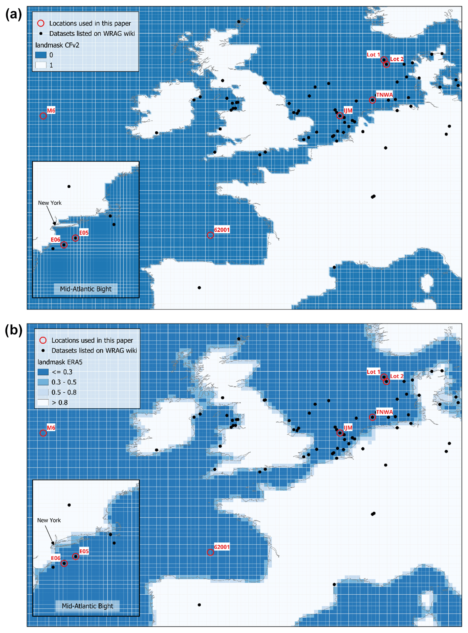
Figure 2Location of the publicly available wind-energy-specific wind datasets (black dots), together with the analysis locations used for this paper. The small box on the bottom left of the subfigures shows the Mid-Atlantic Bight off the USA East Coast, while the larger map shows the North Sea. The two maps show land–sea masks for CFSv2 (a) and ERA5 (b). For ERA5, and for IFS in general, land–sea mask values range from 0 to 1 and indicate (see https://confluence.ecmwf.int/display/FUG/Section+2.1.3.1+Land-Sea+Mask#Section2.1.3.1LandSeaMask-Land-Seamask, last access: 11 August 2024) the fraction of land in the model cell.
All FLS measurements have been validated as per the Carbon Trust Offshore Wind Accelerator Roadmap Stage 3 (Carbon Trust, 2018). That is, both types of lidar and FLS have been validated dozens of times against reference measurements (cups or lidar validated against cups), and these tests have repeatedly shown mean relative deviations smaller than 2 %. Examples of validations are provided in Figs. A1 and A2. A large number of publicly available validation reports have been collected by the authors (see Gandoin, 2024). For the specific case of the Fugro FLS, from the RVO (Rijksdienst voor Ondernemend Nederland (The Netherlands Enterprise Agency)) campaigns (see https://offshorewind.rvo.nl/, last access: 11 August 2024) 16 validation reports are available together with additional studies such as Kelberlau (2022) and Kelberlau and Mann (2022), showing similarly very small deviations against several cup anemometer measurements offshore. For the EOLOS FLS, three validation reports are available in the above-mentioned online repository, and Araújo da Silva et al. (2022) provide a thorough description and validation of the device at the IJmuiden met mast.
All FLSs used in this study are equipped with ZX continuous wave lidars; see Knoop et al. (2021) for a research validation study. The 10 min data have been filtered using a regular filter based on the average number of valid samples during one scan (so-called minimum number of packets); it is here set to 18. Fugro uses a threshold of 9 (see Table 3.2 of Fugro, 2021), and validation studies such as TNO (2021) show that for this type of lidar the accuracy of the measurement is not significantly sensitive to the value of the threshold. A thorough and quantitative overview of availability statistics for these instruments is provided in the references stated in Table 1. For comparisons with model data, the data have been hourly averaged, and only time periods with at least five valid 10 min timestamps have been used.
1.3 Derivation of a 10 m wind time series from measurements
As explained later in Sect. 3.2, when , L and αCh are known, wind speed at any elevation in the surface layer can be computed (an example is given for the 26.1 m cup anemometers at IJmuiden mast (IJM)). Therefore, deriving a 10 m wind from measurement data is not always necessary.
However, for practical reasons this often needs to be done (CFSR and CFSv2 winds are available at 10 m, or, traditionally for spectral wave modelling). In the present article, two methods have been considered for every 10 min timestamp: (1) interpolation using a power law the measurements between the 4 m sonic anemometers and the lowest lidar measurement elevation and (2) fitting of a power or log law to the lidar measurements up to and including 80 m and then extrapolation down to 10 m. Both methods add some uncertainty to the derived 10 m value: for the first the uncertainty mainly lies in the uncertainty of the 4 m sonic anemometers; for the second and in particular for stable conditions, the wind profile may not be well fitted by a power law. To alleviate these uncertainties, the present study focuses on wind speeds higher than 15 and 20 m s−1 (where stable conditions are very rare; this was checked from both reanalysis data time series but also the literature; see Sathe et al., 2011, for the North Sea), and in Sect. 2.3 the comparison is made for unstable and neutral conditions only by limiting the range of air–sea temperature difference to (North Sea) and (Atlantic Bight). The reason for choosing two different ranges of temperature differences is that in the Mid-Atlantic Bight strong wind conditions occur during winter for very unstable conditions. For all these comparisons, the mean wind speed measurement profile is provided to check the validity of the extrapolation method. Furthermore, the uncertainty of the extrapolation method has been verified using proprietary Fugro FLS measurements located in northern Scotland, where 12 m lidar measurements are available (the exact location is confidential): see Fig. 3, which shows that the errors are the smallest when considering method 1). This method has thereby been chosen in Sect. 2.3, but it has been checked that the conclusions of the analysis are not sensitive to the choice of the method (i.e. that the ERA5 10 m wind speeds are lower than measured values, also when considering measurement uncertainty).
Figure 3Panels (a) and (c) show comparisons of 12 m hourly wind speed (WS) measurements from a Fugro FLS (undisclosed location) with 12 m time series derived using the three methods discussed in the text and stated in the legend (PL stands for power law, and LL stands for log law). Panel (a) shows the corresponding mean wind speed profile, where the blue markers are FLS measurements, the black line is the fitted log law and the magenta line is the fitted power law. Measurements have been filtered for 100 m wind speeds (WS100) between 15 and 50 m s−1, as well as for wind directions (WDs) between 270 and 30°.
1.4 Model data
For this study, CFSR (Saha et al., 2010) and CFSv2 (Saha et al., 2014) data have been downloaded using DHI's MetOcean On Demand (MOOD) web interface (see https://www.metocean-on-demand.com/, last access: 11 August 2024, where it is stated that “The data is extracted as discrete (non-interpolated) values of the model grid cell.”). Data from ERA5 (Hersbach et al., 2020) have been downloaded from MOOD as well for the locations M6, Lot 1, Lot 2, E05 and E06. For the locations TNWA (Ten noorden van de Waddeneilanden A, where A is the number of measurement location), IJM and 62001, the ERA5 data were also fetched from the Copernicus Data Store (CDS), and for these locations it was verified that both sources are identical. Compared to in situ measurements, for IJM and TNWA the data were interpolated at the measurement location. For E05, E06, Lot 1 and Lot 2 the nearest node was used. The following parameters have been used (all hourly time series):
-
for CFSR/CFSv2, 10 m wind speed and direction and air and sea surface temperature
-
for ERA5,
-
from Metocean on Demand, 10 and 100 m wind speed and direction
-
from the CDS, same as above plus 2 m air temperature, sea surface temperature, friction velocity, roughness length, Charnock coefficient, sensible heat flux, dew point temperature and pressure at the sea surface.
-
In the literature, multiple comparisons between in situ measurements and IFS model wind speeds close to the surface have concluded that for strong wind conditions the IFS model wind speeds are lower than measured values and lower than other reanalysis datasets (global or regional). See for instance Fery et al. (2018) for ERA Interim and Bentamy et al. (2021), Alday et al. (2021), Solbrekke et al. (2021), Spangehl et al. (2023), and Meyer and Gaslikova (2024) for ERA5.
2.1 Comparisons between ERA5 and CFSv2
Examples of differences with ERA5 (IFS) and CFSv2 (GFS) model results are provided below for two locations: the M6 buoy off the west coast of Ireland and the TNWA FLS (see Fig. 4). Similar trends are visible across several locations on the northwestern European shelf (see the Supplement). Figure 5 shows that at the 62001 buoy location and when separating the dataset between short and long fetches, the relative difference between the models seems to be larger for short fetches; as discussed in Sect. 3 this is a sign that the difference between the models is driven by the dependency of the ERA5 drag formulation to the sea state. In this example, short fetches are defined as wind directions where wind comes from land across the Bay of Biscay, while wind direction oriented towards the Atlantic Ocean is considered long fetches (see Fig. 2). This effect is of the same magnitude at all locations when considering the CFSR data (1 January 1979 to 1 April 2011), which have a coarser resolution than ERA5 (see Gandoin, 2024).
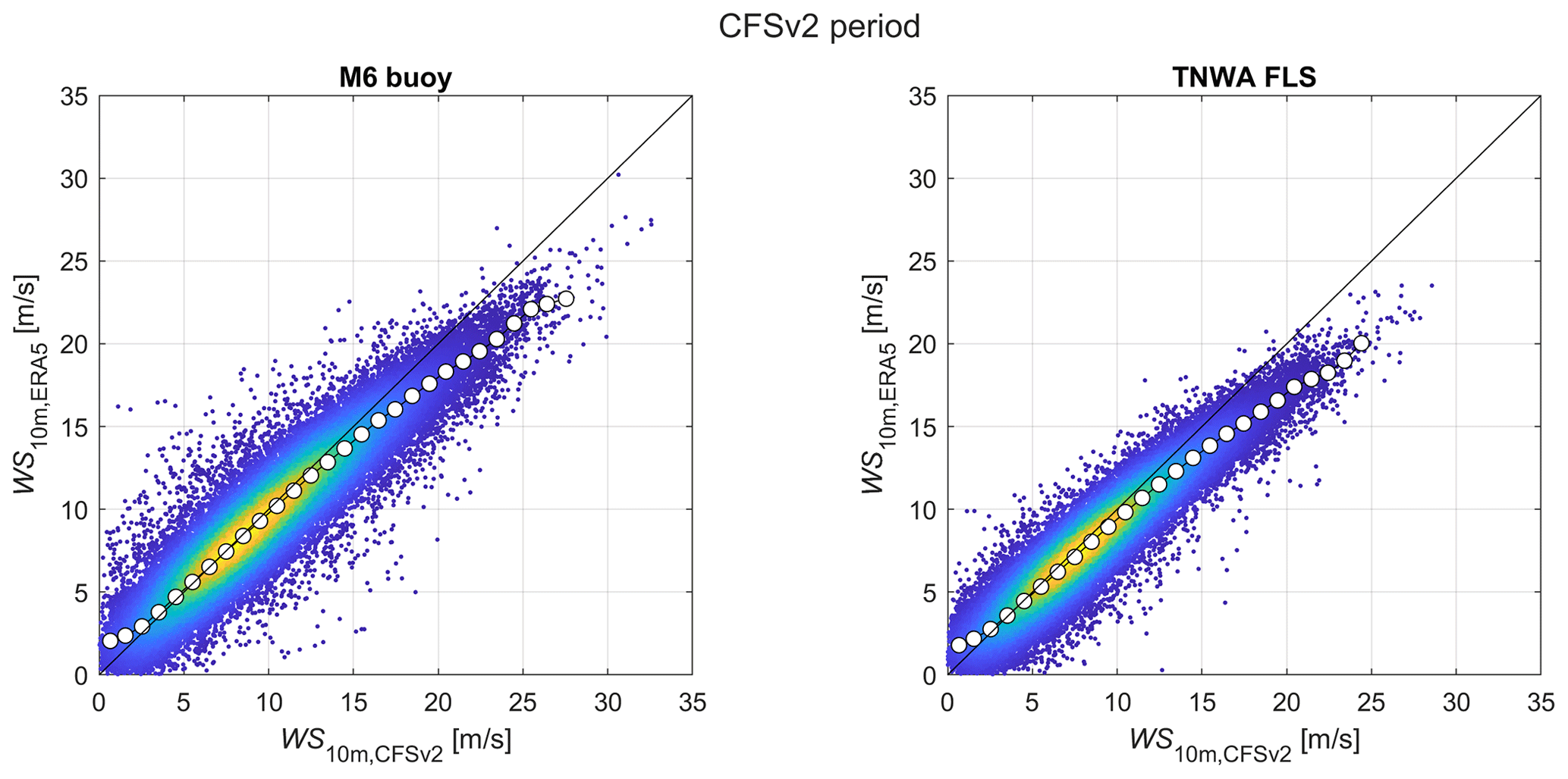
Figure 4For two locations (see Fig. 2), comparison of the ERA5 and CFSv2 10 m wind speeds. For wind speeds above approximately 10 m s−1, the ERA5 values are smaller than the CFSv2 values; this effect is stronger at TNWA than at M6. The density of the scatterplot uses a colour map, from blue (low density, few points) to yellow (high density, many points). The white dots are the binned mean values (for bins with more than 10 points).
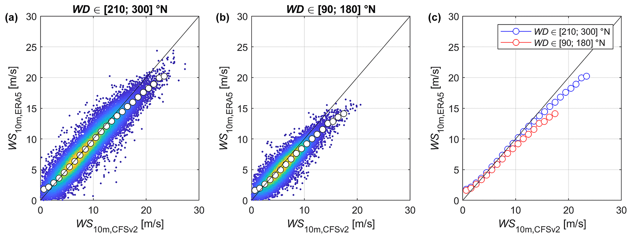
Figure 5As for Fig. 4, this figure shows a comparison of ERA5 and CFSv2 10 m wind speeds, this time at the 62001 buoy and for two wind directional bins corresponding to a very long fetch and a short fetch. The difference between the two model results is larger for short fetches. The white dots are the binned mean values (for bins with more than 10 points).
2.2 Comparisons between ERA5 and measurements
Using the method explained in Sect. 1.3, 10 m wind speed time series have been derived from FLS measurements. These values were compared with ERA5 and CFSv2 model data for five measurement locations in Fig. 6 (Lot 1) and in Figs. A3–A6. For all locations, the ERA5 values are smaller than the measured values and smaller than the CFSv2 values.
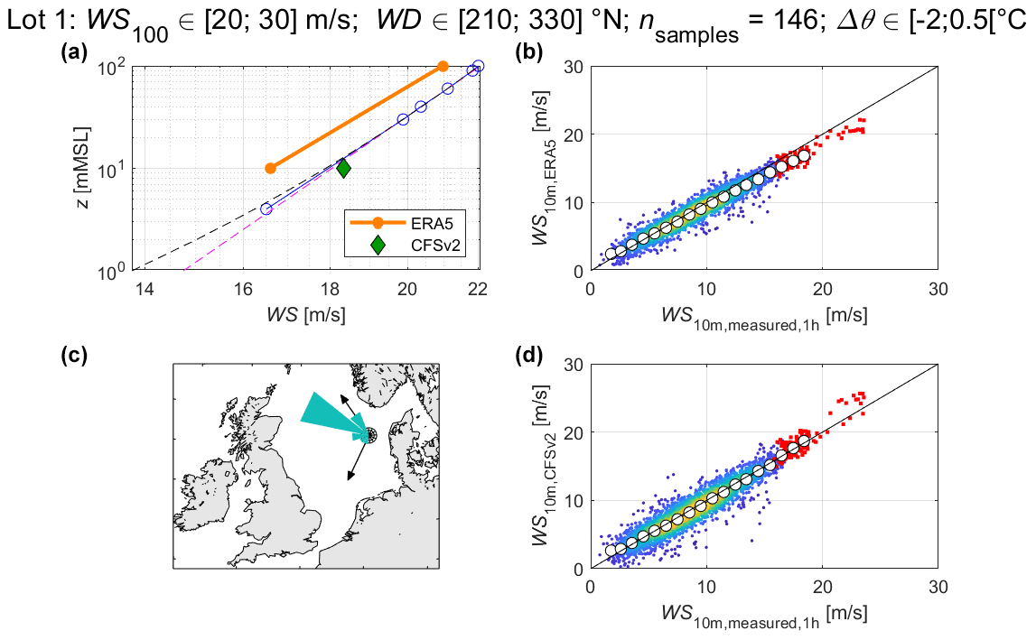
Figure 6For one FLS location in the Danish North Sea, comparison between modelled and measured hourly mean wind speeds. The white dots are the binned mean values (for bins with more than 10 points). A subset of high wind speeds (selected using the FLS measurements at 100 m) are highlighted in red. The plot to the top left shows mean wind speed profiles for this subset, where the blue line represents measurements. The dashed black line is a power law fit to the measurement data below 80 m; the magenta line represents a log law. The 10 m measured data on the x axis of the scatterplots have been interpolated between the 4 m sonic anemometer and the lowest lidar elevation; it can be checked on the top left that this is a valid approach that introduces an uncertainty smaller than the difference between the two models. A wind rose corresponding to the subset of high wind speeds (in red on the scatterplots) is shown on the map.
In Sect. 3.1, using ERA5 data downloaded from the CDS, we check that ERA5 wind speeds can be derived from friction velocity, Charnock parameter and the Obukhov length; then we analyse the behaviour of the ERA5 drag formulation for different sea state conditions and conclude that the ERA5 bias likely comes from the asymptotic behaviour of Eq. (3) for large values of . Then, in Sect. 3.2 we propose a simple correction which consists of capping, or keeping constant, the values of the Charnock parameter.
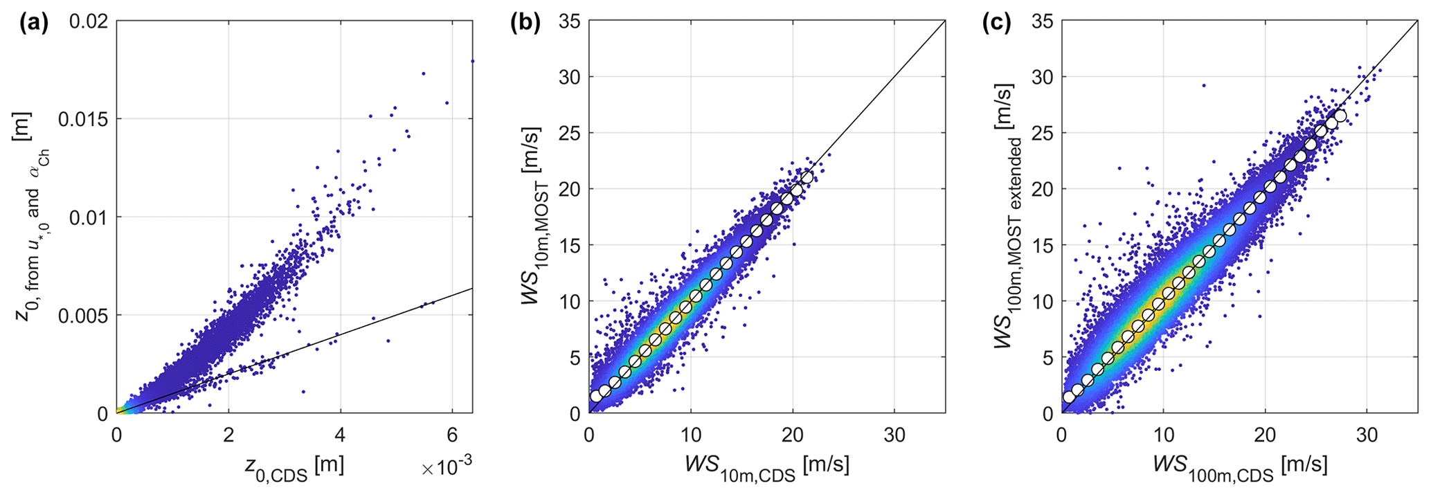
Figure 7For ERA5 at the TNWA location, the left-hand side of this figure shows comparisons between the roughness length values from the CDS (faulty) and the ones computed using the friction velocity and the Charnock parameter time series. The plot in the middle shows a comparison between the 10 m wind speed from the CDS and the one derived using MOST with the friction velocity, the roughness length derived from friction velocity and Charnock parameter, and the Obukhov length computed from CDS time series. The plot to the right shows a comparison between the 100 m wind speed time series from the CDS and the one derived from the same parameters as for the middle plot, plus the surface layer extension model from Gryning et al. (2007). The white dots are the binned mean values (for bins with more than 10 points). Overall, this figure shows that the wind speed values from the CDS at 10 and 100 m can easily be reproduced using well-known wind profile expressions.
3.1 Drag formulation in ERA5
As explained in Sect. 1, friction velocity, roughness length and mean wind speed are interlinked via Eqs. (1) and (2). On the one hand, the ERA5 analysis 10 m wind speed time series is readily available (via its two horizontal components) on the CDS. On the other hand, friction velocity u∗0 and roughness length z0 are only provided as forecast values. Please note that this forecast roughness length time series is faulty and should not be used (Item 18 on https://confluence.ecmwf.int/display/CKB/ERA5:+data+doc umentation#ERA5:datadocumentation-Knownissues, last access: 11 August 2024); instead, the best way to estimate z0 from CDS data is to use the Charnock coefficient time series (available from the CDS) and as in Eq. (2). As a result, ERA5 10 m wind speed time series can be reconstructed solely using Eq. (1) with , αCh and L computed from CDS data.1 As shown in Fig. 7 this gives satisfactory results. Furthermore, the formulations presented in Gryning and al. (2007) can be used to derive very realistic 100 m wind speeds; see Fig. 7 as well (this is helpful to practitioners who may want to derive wind speeds at higher elevations). As explained above, is provided as a forecast value, while the 10 m wind speed from the CDS comes from the analysis (ERA5 contains both analysis and forecast fields); also, the Obukhov length L is computed from other model fields and does not necessarily correspond, for every timestamp, to the value used in the IFS. These differences explain the scatter between the reconstructed 10 m wind speeds and the ones from the CDS, in the second plot in Fig. 7.
3.2 Bias explanation and correction
From the above discussion, the results of the ERA5 drag formulation can be analysed further, with regards to Eq. (3) and the sea state dependency of the Charnock parameter. For increasing values of , the resulting value of z0 has been computed for a wide range of 10 m wind speeds using Eqs. (1) and (2) iteratively, and the results are shown against ERA5 time series at TNWA and the 62001 buoy in Fig. 8. For strong wind speeds the z0 values are relatively larger for the former than for the latter, and for large values of , small changes of this ratio lead to very large changes in z0: for instance, at 15 m s−1, a change from 0.99 to 0.995 in leads to a 60 % increase in z0. Since, as shown in Fig. 9, the ERA5- and CFSR/CFSv2-derived friction velocity values are similar, this increase in roughness length leads to a decrease in mean wind speed.
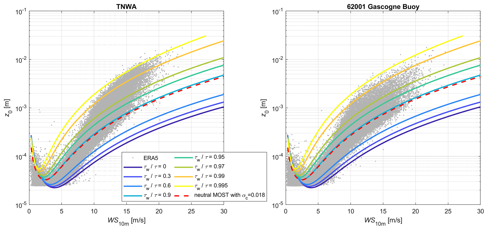
Figure 8For two locations, this figure shows a scatterplot of ERA5 roughness lengths values against 10 m wind speed. Using an iterative process, Eqs. (1)–(3) have been solved for different values of ratios between wave and wind stress and for a constant Charnock parameter value of 0.018. The results are shown in the figures.
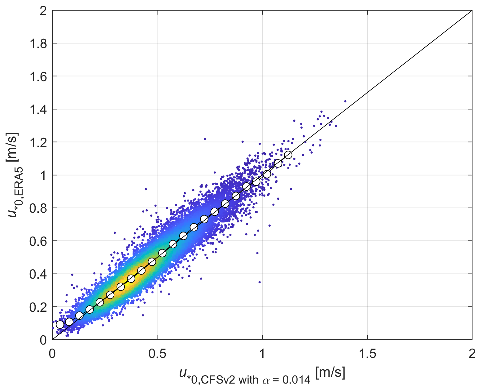
Figure 9For the TNWA FLS location and for neutral conditions, this figure shows a comparison between friction velocities values from the ERA5 and the ones derived iteratively using Eqs. (1) and (2) and the 10 m CFSv2 wind speed time series (with a constant Charnock coefficient of 0.014; see Renfrew et al., 2002). The white dots are the binned mean values (for bins with more than 10 points).
In IFS, as increases, the Charnock coefficient increases; Fig. 10 shows that this is particularly the case for short-fetch conditions in relatively shallow waters like the North Sea. For such conditions and for a given value of significant wave height, the peak period of the spectra is typically smaller than for fully developed, long-fetch conditions. The bias in IFS may then be related to the growth rate parameterisation described in Sect. 2.2 of ECMWF (2016b). This should be investigated in future works, for instance in ERA6 and ERA7 pre-production validation studies (see Sect. 4).
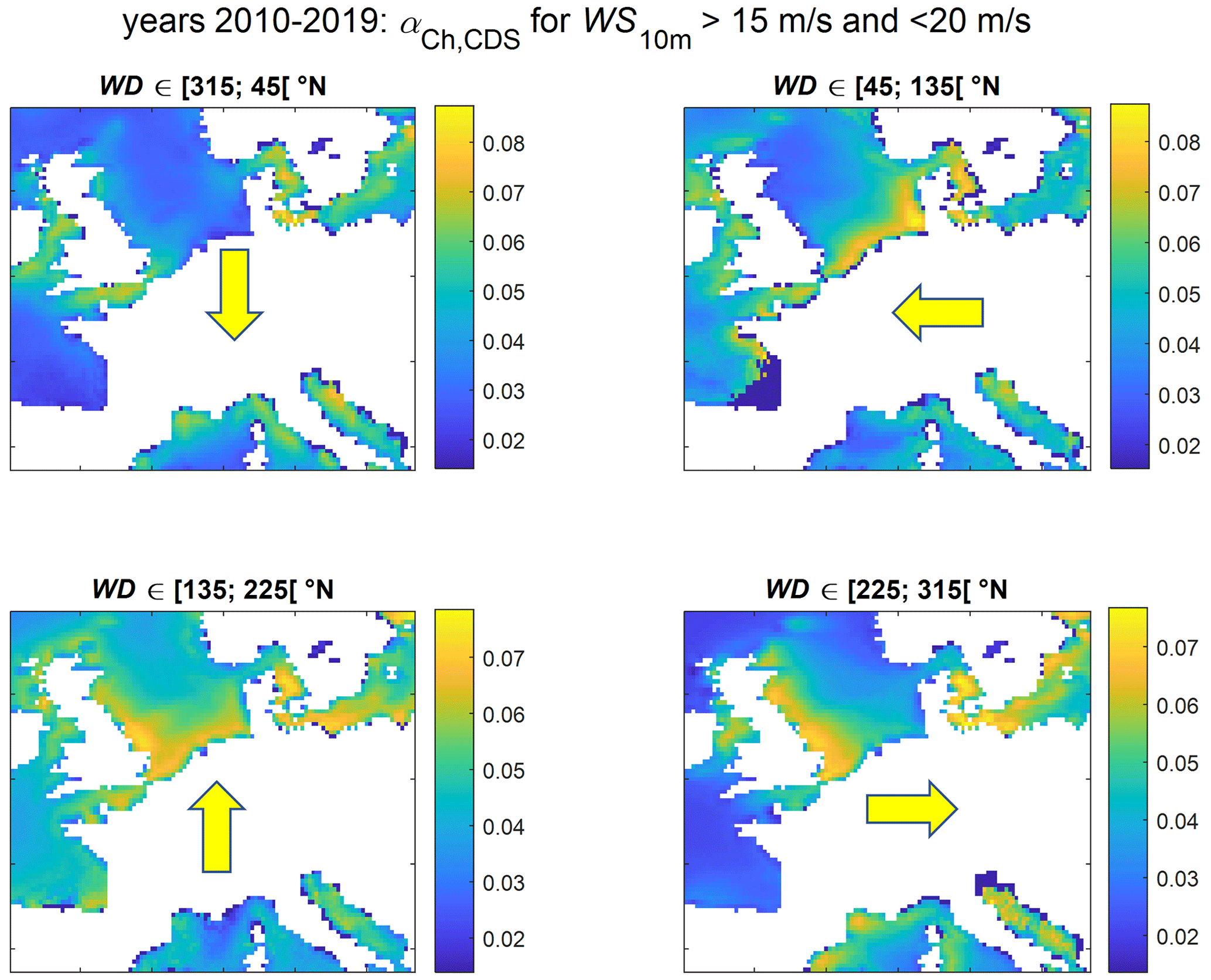
Figure 10This figure shows mean values of ERA5 Charnock coefficient for strong wind speed conditions and four different wind directional bins. The filters have been applied for each ERA5 node: the timestamps selected for computing the Charnock coefficient values are not necessarily concurrent between all the nodes.
3.3 Bias correction
From the above, we conclude that CFSv2 and ERA5 can come to a closer agreement when changing the value of the ERA5 Charnock parameter. This is demonstrated in Fig. 11, where ERA5 αCh values are set to 0.018, and 10 m ERA5 wind speeds are derived as explained in the previous section. The value of 0.018 has been chosen empirically by the authors of the report, from experience and preparatory works (published on https://eo-winds.net/2021/09/06/reconciling-surface-layers-wind-speeds-in-cfs-and-era5, last access: 11 August 2024). Other values reported in the literature include 0.012 in Araújo da Silva et al. (2022), 0.012 to 0.014 in Peña and Gryning (2008), and 0.018 for the IFS ran without the ocean model (see https://codes.ecmwf.int/grib/param-db/148, last access: 11 August 2024) and in Brown et al. (2013). Please note that the MOST should be used to obtain satisfactory results for mow to moderate wind speeds where atmospheric stability is important, i.e. using the Obukhov length as explained in Sect. 3.1.
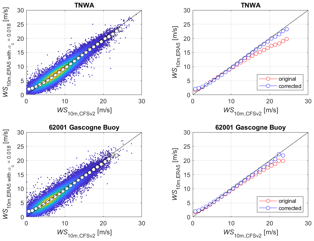
Figure 11This figure shows a comparison of ERA5 10 m wind speeds computed, as explained the text, using the CDS friction velocity and Charnock parameter capped at 0.018 and the CFSv2 time series. The white dots are the binned mean values (for bins with more than 10 points). This method greatly reduced the difference at high wind speeds.
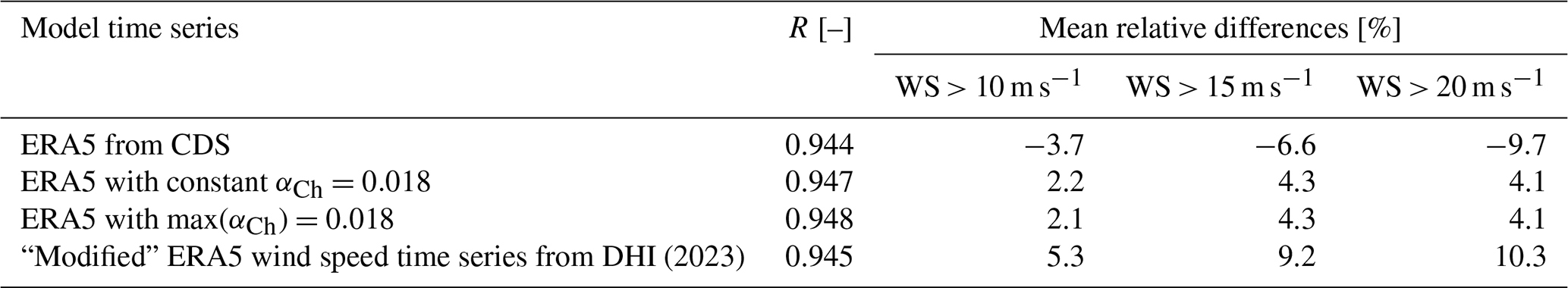
Furthermore, this methods allows a direct comparison of ERA5 values with measurements, without having to extrapolate the measurement elevation: see the example of the 26.1 m anemometer time series at the IJmuiden mast in Fig. 12, where four time series are compared: original ERA5 (top left), ERA5 with constant αCh=0.018 (top right), ERA5 with max(αCh)=0.018 (bottom left) and the method employed in the Global Atlas of Siting Parameters Ocean and Coast (GASPOC) project (DHI, 2023) for their “modified” ERA5 wind speed time series (bottom right). This last method uses ERA5 wind speed and atmospheric stability information only (not αCh nor ), and it leads therefore to higher wind speeds in strong wind conditions. The method where αCh is capped to 0.018 is analogous to reduced drag methods commonly used for ocean surface layer modelling; see for instance Sect. 2.6 of DHI (2017) or the SWAN model documentation (see https://swanmodel.sourceforge.io/online_doc/swantech/node15.html, last access: 2 May 2024). As shown in Table 2, the suggested correction method (constant αCh=0.018 or max(αCh)=0.018) leads to a slight overestimation of strong wind speeds, while the original ERA5 data show an underestimation of almost 10 % for the largest values.
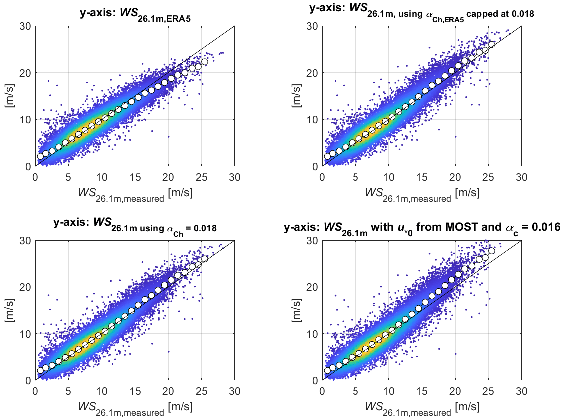
Figure 12This figure shows a comparison of ERA5 26.1 m wind speeds and measurements at 26.1 m from the IJmuiden mast. The model data are computed as explained the text and summarised in the title of the subplots. The white dots are the binned mean values (for bins with more than 10 points).
Table 2Pairwise linear correlation coefficient R and mean relative differences between the four model time series described in the text and hourly wind speed measurements at IJM (26.1 m a.m.s.l.). The mean relative differences are computed for three different thresholds of measured wind speeds.
3.4 Limitations and applicability of the proposed methodology
The suggested correction method presented earlier is not free from limitations. In this section, we discuss four main topics which should be investigated further: (a) the choice of the Charnock parameter, (b) the validity of the method for wind speeds higher than 25 m s−1, (c) the derivation of wind speed values for shorter averaging period than 1 h and (d) validation for long fetches.
As explained in Sect. 1.1, all the drag formulations presented in this study require some degree of tuning using one or more empirical parameters. In our case, we propose a single value of the Charnock parameter, 0.018, which gives satisfactory results for correcting ERA5 wind speeds so that they match CFSR/CFSv2 values (the industry-preferred model; see Sect. 1) as well as measurements. For a given offshore wind project, the practitioner may change or adapt this value to best fit their objectives, and the choice of this parameter should always be documented, discussed and contextualised.
Our measurement datasets do not contain 10 m hourly wind speeds higher than 25 m s−1. For tropical cyclone conditions where 10 m wind speeds can exceed 30 m s−1, judging from the results presented in Janssen and Bidlot (2023) and Bouin et al. (2024) about drag coefficient reduction at such high wind speeds, the proposed method likely overestimates measured values.
For engineering applications, it is often necessary to assess extreme values for averaging times shorter than 1 h: typically 10 min, 1 min and 3 s. The IFS and GFS NWP modelling systems do not explicitly model microscale turbulent eddies and therefore rely on parameterisations; see Sect. 3.10.4 of ECMWF (2016a). In engineering, measurement-based methods are used (Andersen and Løvseth, 2006), alongside model-based, empirical spectral correction methods (Larsén and Ott, 2022). Our correction method only deals with 1 h wind speeds; for deriving shorter averaging we refer to the two above-mentioned studies.
Finally, our study does not show a validation for long-fetch conditions, where, as shown in Fig. 5, differences between CFSR/CFSv2 and ERA5 are smaller. This is because the measurement datasets currently publicly available are primarily in enclosed seas or in places where the strongest 10 m winds come from the shore. There exist high-quality lidar measurements in the open ocean, but they are not publicly available. When such datasets become publicly available or for projects with such data, additional validations should be carried out.
Overall, it important to stress that our study does not conclude that using an uncoupled version of IFS, with a constant Charnock parameter, is preferable to using a coupled model. In effect, there are many advantages to using a coupled model as it reflects more truly the nature of air–sea interactions. Yet, for specific applications and regions, biases can appear, and we wish to demonstrate that, with all the necessary information, simple and transparent correction methods can be derived.
The characterisation of the interactions between wind, sea state and currents remains an active field of research. Flux measurement experiments have been carried out only at a few locations, and the theoretical basis for understanding these interactions is still in development (Ayet and Chapron, 2022; Janssen and Bidlot, 2023).
Modellers have adapted these models to one- or two-way coupled atmosphere–ocean modelling systems, and comparisons are regularly performed; see for instance Edson et al. (2013) and Bouin et al. (2024). These comparisons are often carried out for locations that are not representative of offshore wind locations. For instance, the ECMWF drag formulation in Edson et al. (2013) is representative of the “globally averaged wave age-dependent roughness at a given wind speed”. As oceans cover 70 % of the world, these model grid cells are for the most part deep-water, very far offshore locations where the fetch- and bathymetry-dependent bias discussed in Sect. 3 is less visible. Alternatively, in Bouin et al. (2024) and Janssen and Bidlot (2023), the focus is on very high wind speeds during tropical cyclones (TCs). This is of value to the forecasting community, but offshore wind applications require the entire range of wind speeds to be modelled accurately.
Some may argue that when focusing on modelling sea state hydrodynamic conditions, adjustments to the wind forcing are as equally important as the other wave spectra sources and sinks of energy (bottom friction, wave–wave interactions etc.). This is true, but the end users and in particular offshore wind practitioners require both wind and waves/hydrodynamics to be correct. As the next generation of high-resolution (towards kilometre-scale) reanalysis datasets are being prepared for production (ERA6/7, MERRA-3), planning for sector or class of user-specific validations becomes necessary, for instance with increasing complexity:
-
Validation runs against mast, lidar and FLS measurements during a great number of storm events (this is commonly done for commercial projects). Adding such datasets alongside legacy measurements such as met buoys would prove very valuable and persuasive for wind energy practitioners. On the other hand, oceanographers who are relying in legacy measurement would find an alternative, higher-quality dataset to work with.
-
Refined grid meshes are in coastal areas where offshore wind projects are being developed and are adapting model data delivery to the needs of offshore wind practitioners.
-
Lidar measurements should be included in air–sea interaction measurement campaigns (as in the WFIP3 project; see https://www.psl.noaa.gov/renewable_energy/wfip3/, last access: 11 August 2024).
-
Work should continue towards unifying oceanographic and ABL meteorology frameworks, from a wind energy perspective as discussed in Shaw et al. (2022).
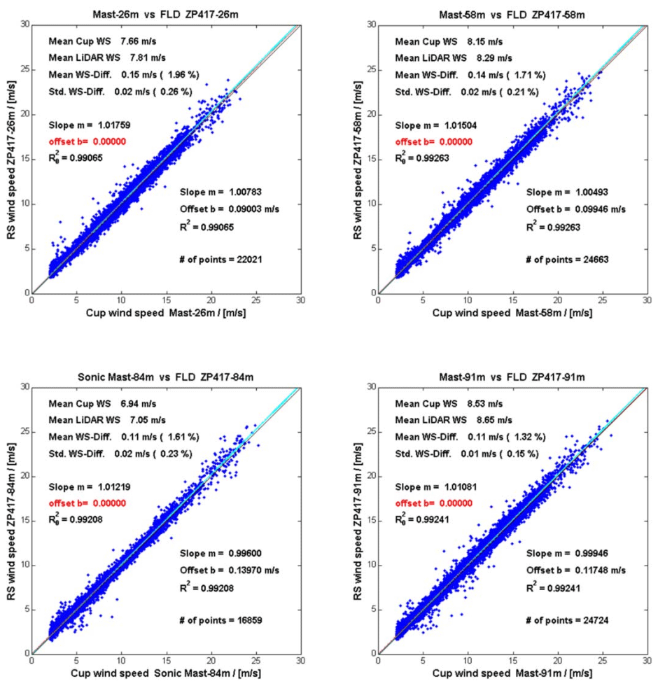
Figure A1Example of FLS lidar validation (from GLGH, 2015).
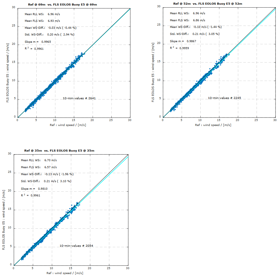
Figure A2Example of FLS validation (from DNV GL, 2019).
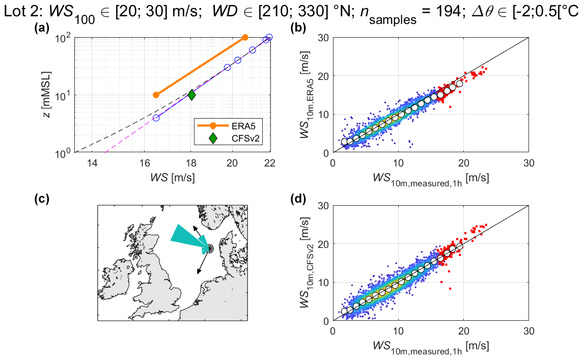
Figure A3Same as Fig. 6 but for the Lot2 FLS location in the Danish North Sea.
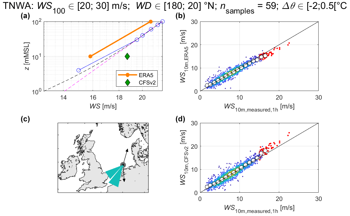
Figure A4Same as Fig. 6 but for the TNWA location in the Danish North Sea.
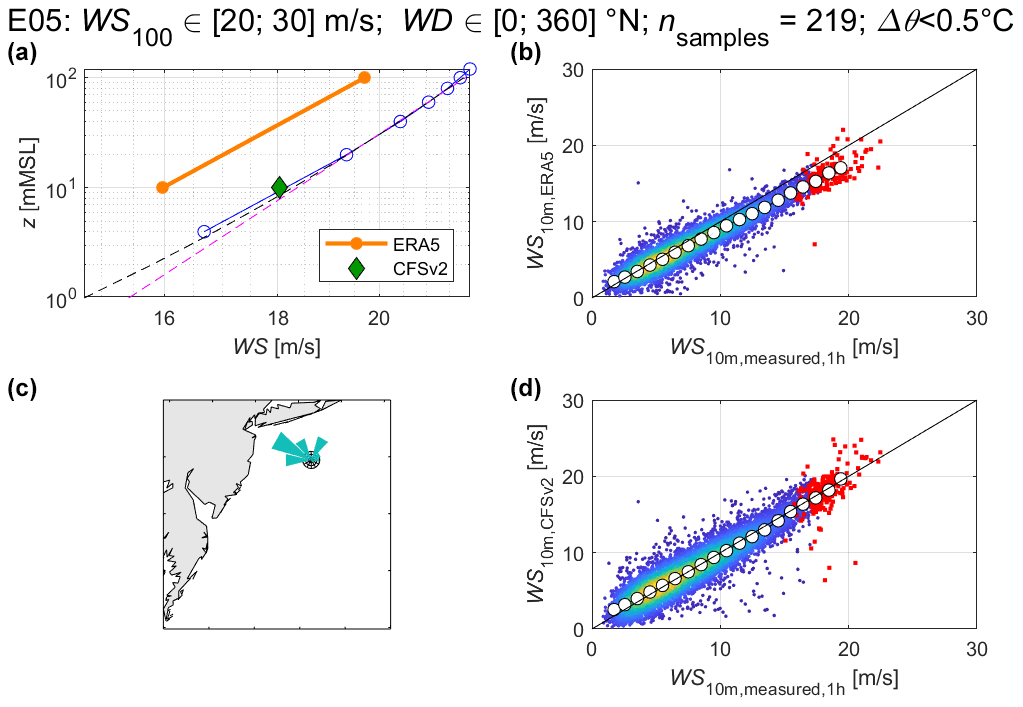
Figure A5Same as Fig. 6 but for the E05 FLS location in the New York Bight.
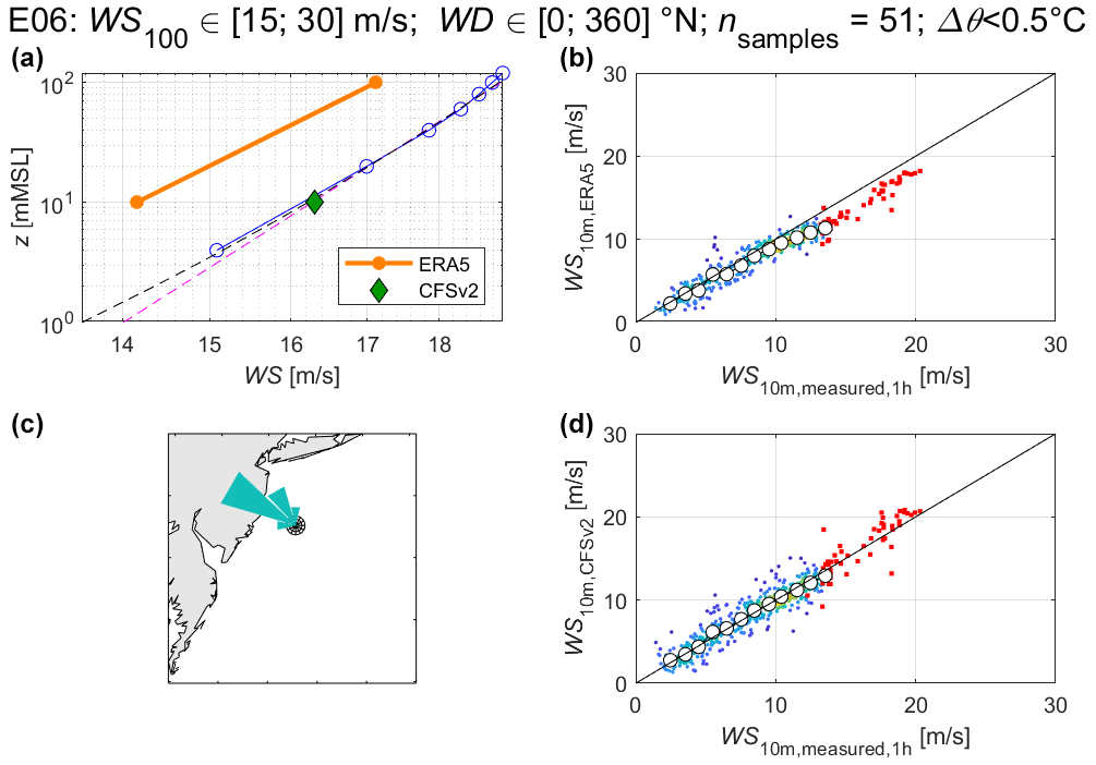
Figure A6Same as Fig. 6 but for the E06 FLS location in the New York Bight.
The code is not available, as some of the functions are property of C2Wind ApS. The data are publicly available; see Saha et al. (2010, https://doi.org/10.1175/2010BAMS3001.1), Saha et al. (2014, https://doi.org/10.1175/JCLI-D-12-00823.1), Hersbach et al. (2020, https://doi.org/10.1002/qj.3803), https://offshorewind.rvo.nl/ (RVO, 2024), https://oswbuoysny.resourcepanorama.dnv.com/ (DNV, 2024), https://www.metocean-on-demand.com/ (DHI, 2024), and https://ens.dk/en/our-responsibilities/offshore-wind-power/preliminary-site-investigations-energy-islands (ENS, 2024).
Publicly available lidar and FLS validation reports, as well as comparisons of ERA5 and CFSR/CFSv2 10 m wind speeds at several locations, are provided in Zenodo (https://doi.org/10.5281/zenodo.11100768, Gandoin, 2024).
RG conceptualised the article and carried out the analysis. JG reviewed the manuscript.
The contact author has declared that neither of the authors has any competing interests.
Publisher's note: Copernicus Publications remains neutral with regard to jurisdictional claims made in the text, published maps, institutional affiliations, or any other geographical representation in this paper. While Copernicus Publications makes every effort to include appropriate place names, the final responsibility lies with the authors.
The authors would like thank Jean Bidlot for his patience and his interest in offshore wind applications.
This paper was edited by Atsushi Yamaguchi and reviewed by two anonymous referees.
Alday, M., Accensi, M., Ardhuin, F., and Dodet, G.: A global wave parameter database for geophysical applications, Part 3: Improved forcing and spectral resolution, Ocean Model., 166, 101848–10167, https://doi.org/10.1016/j.ocemod.2021.101848, 2021.
Andersen, O. J. and Løvseth, J., The Frøya database and maritime boundary layer wind description, Mar. Struct., 19, 173–192, https://doi.org/10.1016/j.marstruc.2006.07.003, 2006.
Araújo da Silva, M. P., Rocadenbosch, F., Farré-Guarné, J., Salcedo-Bosch, A., González-Marco, D., and Peña, A.: Assessing Obukhov Length and Friction Velocity from Floating Lidar Observations: A Data Screening and Sensitivity Computation Approach, Remote Sens., 14, 1394, https://doi.org/10.3390/rs14061394, 2022.
Ayet, A. and Chapron, B.: The dynamical coupling of wind-waves and atmospheric turbulence: a review of theoretical and phenomenological models, Bound.-Lay. Meteorol., 183, 1–33, https://doi.org/10.1007/s10546-021-00666-6, 2022.
Bentamy, A., Grodsky, S. A., Cambon, G., Tandeo, P., Capet, X., Roy, C., Herbette, S., and Grouazel, A.: Twenty-Seven Years of Scatterometer Surface Wind Analysis over Eastern Boundary Upwelling Systems, Remote Sens., 13, 940, https://doi.org/10.3390/rs13050940, 2021.
Bouin, M.-N., Lebeaupin Brossier, C., Malardel, S., Voldoire, A., and Sauvage, C.: The wave-age-dependent stress parameterisation (WASP) for momentum and heat turbulent fluxes at sea in SURFEX v8.1, Geosci. Model Dev., 17, 117–141, https://doi.org/10.5194/gmd-17-117-2024, 2024.
Brown, J. M., Amoudry, L. O., Mercier, F. M., and Souza, A. J.: Intercomparison of the Charnock and COARE bulk wind stress formulations for coastal ocean modelling, Ocean Sci., 9, 721–729, https://doi.org/10.5194/os-9-721-2013, 2013.
Carbon Trust: Carbon Trust Offshore Wind Accelerator Roadmap for Commercial Acceptance of Floating LiDAR Technology, Version 2.0, https://www.carbontrust.com/our-work-and-impact/guides-reports-and-tools/roadmap-for-commercial-acceptance-of-floating-lidar (last access: 11 August 2024), 2018.
DHI: MIKE 21 & MIKE 3 Flow Model FM, Hydrodynamic and Transport Module, Scientific Documentation, https://manuals.mikepoweredbydhi.help/2017/Coast_and_Sea/MIKE_321_FM_Scientific_Doc.pdf (last access: 11 August 2024), 2017.
DHI: EUDP Global Atlas of Siting Parameters Offshore, ERA5 Wind: Validation and Comparison, Report, https://www.metocean-on-demand.com/metadata/waterdata-dataset-Global_ERA5 (last access: 11 August 2024), 2023.
DHI: MetOcean Data Portal, https://www.metocean-on-demand.com/, last access: 11 August 2024.
DNV GL: Assessment of EOLOS FLS-200 E05 Floating Lidar Pre-Deployment Validation at the Narec NOAH Offshore Met Tower, UK, Report No. 02, Rev. A, Document No. 10124962-R-2-A, https://oswbuoysny.resourcepanorama.dnv.com/download/f67d14ad-07ab-4652-16d2-08d71f257da1 (last access: 11 August 2024), 2019.
DNV: NYSERDA Floating LiDAR Buoy Data, https://oswbuoysny.resourcepanorama.dnv.com/, last access: 11 August 2024.
ENS: Preliminary site investigations for the Energy Islands, https://ens.dk/en/our-responsibilities/offshore-wind-power/preliminary-site-investigations-energy-islands, last access: 15 August 2024.
ECMWF: IFS Documentation – Cy41r2, Operational implementation 8 March 2016, Part IV: Physical Processes, https://doi.org/10.21957/tr5rv27xu, 2016a.
ECMWF: IFS Documentation – Cy41r2, Operational implementation 8 March 2016, Part VII: ECMWF Wave Model, https://doi.org/10.21957/672v0alz, 2016b.
Edson, J. B., Jampana, V., Weller, R. A., Bigorre, S. P., Plueddemann, A. J., Fairall, C. W., Miller, S. D., Mahrt, L., Vickers, D., and Hersbach, H.: On the Exchange of Momentum over the Open Ocean, J. Phys. Oceanogr., 43, 1589–1610, https://doi.org/10.1175/JPO-D-12-0173.1, 2013.
ENTSO-E: TYNDP 2024, Offshore Network Development Plans European offshore network transmission infrastructure needs, Pan-European summary, https://eepublicdownloads.blob.core.windows.net/public-cdn-container/tyndp-documents/ONDP2024/ONDP2024-pan-EU-summary.pdf (last access: 11 August 2024), 2024.
EOLOS: NYSERDA Measurement Plan, Code: EOL-NYS01, Revision 02, https://oswbuoysny.resourcepanorama.dnv.com/download/f67d14ad-07ab-4652-16d2-08d71f257da (last access: 11 August 2024), 2020.
Fery, N., Tinz, B., Ganske, A., and Gates, L.: Reproduction of 10 m-wind and sea level pressure fields during extreme storms with regional and global atmospheric reanalyses in the North Sea and the Baltic, in: 2nd Baltic Earth Conference, Helsingør, 11–15 June 2018, https://doi.org/10.13140/RG.2.2.24884.35200, 2018.
Fugro: Supply of Meteorological and Oceanographic data at Hollandse Kust (west), 24-month summary campaign report: 5 February 2019–11 February 2021, Fugro Document No. C75432_24M_F, https://offshorewind.rvo.nl/file/download/498241e9-bdb1-45ce-8343-303727e620a7/1639050959hkw_20211125_mc_fugro_24m report_f.pdf (last access: 11 August 2024), 2021.
Fugro: Supply of Meteorological and Oceanographic data at Ten noorden van de Waddeneilanden 24-month summary campaign report: 19 June 2019–20 June 2021, Fugro Document No. C75433_24M_F, https://offshorewind.rvo.nl/file/download/3b2f655f-af72-4bf5-9754-a7d2d2e6dc6c/tnw_20220118_mc_fugro_report-f.pdf (last access: 11 August 2024), 2022.
Fugro: SWLB measurements at Energy Islands. Project Measurement Plan, All Lots, C75486_Project_Measurement_Plan_All_Lots 09, Final, ENS's FTP, https://ens.dk/en/our-responsibilities/offshore-wind-power/preliminary-site-investigations-energy-islands-0 (last access: 11 August 2024), 2023.
Gandoin, R.: Supplementary material to the Wind Energy Science article “Underestimation of strong wind speeds offshore in ERA5: evidence, discussion, and correction”, Version v2, Zenodo [data set], https://doi.org/10.5281/zenodo.11100768, 2024.
GLGH: Assessment of the Fugro/Oceanor Seawatch Floating LiDAR Verification at RWE IJmuiden met mast, Technical Note No. GLGH-4257 13 10378-R-0003, Rev. B, https://offshorewind.rvo.nl/file/download/ae688c2d-721f-416c-8902-51f0c0f5bf63/1502435907hkz_20150130_dnvgl_ijmuiden trial campaign validation-f.pdf (last access: 11 August 2024), 2015.
Gryning, S.-E., Batcharova, E., Brümmer, B., Jørgensen, H., and Larsen, S.: On the extension of the wind profile over homogeneous terrain beyond the surface boundary layer, Bound.-Lay. Meteorol., 124, 251–268, https://doi.org/10.1007/s10546-007-9166-9, 2007.
Hersbach, H., Bell, B., Berrisford, P., et al.: The ERA5 global reanalysis, Q. J. Roy. Meteorol. Soc., 146, 1999–2049, https://doi.org/10.1002/qj.3803, 2020.
Janssen, P. A. E. M. and Bidlot, J.: Wind–Wave Interaction for Strong Winds, J. Phys. Oceanogr., 53, 779–804, https://doi.org/10.1175/JPO-D-21-0293.1, 2023.
Kelberlau, F.: Floating Lidar Systems, Measurement accuracy under strong wind conditions, in: WRM Discussion group meeting, 30 March 2022, https://oceanalysis-my.sharepoint.com/:f:/p/gus_jeans/Ep9M6eSQXPZLl9-fNpZ_7mMBDpRKZ8KEu_yXoMeN5e5ZdQ (last access: 11 August 2024), 2022.
Kelberlau, F. and Mann, J.: Quantification of motion-induced measurement error on floating lidar systems, Atmos. Meas. Tech., 15, 5323–5341, https://doi.org/10.5194/amt-15-5323-2022, 2022.
Knoop, S., Bosveld, F. C., de Haij, M. J., and Apituley, A.: A 2-year intercomparison of continuous-wave focusing wind lidar and tall mast wind measurements at Cabauw, Atmos. Meas. Tech., 14, 2219–2235, https://doi.org/10.5194/amt-14-2219-2021, 2021.
Larsén, X. G. and Ott, S.: Adjusted spectral correction method for calculating extreme winds in tropical-cyclone-affected water areas, Wind Energ. Sci., 7, 2457–2468, https://doi.org/10.5194/wes-7-2457-2022, 2022.
Meyer, E. M. I. and Gaslikova, L.: Investigation of historical severe storms and storm tides in the German Bight with century reanalysis data, Nat. Hazards Earth Syst. Sci., 24, 481–499, https://doi.org/10.5194/nhess-24-481-2024, 2024.
Peña, A. and Gryning, S. E.: Charnock's Roughness Length Model and Non-dimensional Wind Profiles Over the Sea, Bound.-Lay. Meteorol., 128, 191–203, https://doi.org/10.1007/s10546-008-9285-y, 2008.
Peña, A., Gryning, S.-E., and Hasager, C.: Measurements and Modelling of the Wind Speed Profile in the Marine Atmospheric Boundary Layer, Bound.-Lay. Meteorol., 129, 479–495, https://doi.org/10.1007/s10546-008-9323-9, 2008.
Pineau-Guillou, L., Ardhuin, F., Bouin, M.-N., Redelsperger, J.-L., Chapron, B., Bidlot, J.-R., and Quilfen, Y.: Strong winds in a coupled wave–atmosphere model during a North Atlantic storm event: evaluation against observations, Q. J. Roy. Meteorol. Soc., 144, 317–332, https://doi.org/10.1002/qj.3205, 2018.
Quaeghebeur, E. and Zaaijer, M. B.: How to improve the state of the art in metocean measurement datasets, Wind Energ. Sci., 5, 285–308, https://doi.org/10.5194/wes-5-285-2020, 2020.
Ramon, J., Lledó, L., Torralba, V., Soret, A., and Doblas-Reyes, F. J.: What global reanalysis best represents near-surface winds?, Q. J. Roy. Meteorol. Soc., 145, 3236–3251, https://doi.org/10.1002/qj.3616, 2019.
Renfrew, I. A., Moore, G. W. K., Guest, P. S., and Bumke, K.: A Comparison of Surface Layer and Surface Turbulent Flux Observations over the Labrador Sea with ECMWF Analyses and NCEP Reanalyses, J. Phys. Oceanogr., 32, 383–400, https://doi.org/10.1175/1520-0485(2002)032<0383:ACOSLA>2.0.CO;2, 2002.
RVO: https://offshorewind.rvo.nl/, last access: 11 August 2024.
Saha, S., Moorthi, S., Pan, H.-L. et al.: The NCEP Climate Forecast System Reanalysis, B. Am. Meteorol. Soc., 91, 1015–1058, https://doi.org/10.1175/2010BAMS3001.1, 2010.
Saha, S., Moorthi, S., Wu, X. et al.: The NCEP Climate Forecast System Version 2, J. Climate, 27, 2185–2208, https://doi.org/10.1175/JCLI-D-12-00823.1, 2014.
Sathe, A., Gryning, S.-E., and Peña, A.: Comparison of the atmospheric stability and wind profiles at two wind farm sites over a long marine fetch in the North Sea, Wind Energy, 14, 767–780, https://doi.org/10.1002/we.456, 2011.
Shaw, W. J., Berg, L. K., Debnath, M., Deskos, G., Draxl, C., Ghate, V. P., Hasager, C. B., Kotamarthi, R., Mirocha, J. D., Muradyan, P., Pringle, W. J., Turner, D. D., and Wilczak, J. M.: Scientific challenges to characterizing the wind resource in the marine atmospheric boundary layer, Wind Energ. Sci., 7, 2307–2334, https://doi.org/10.5194/wes-7-2307-2022, 2022.
Solbrekke, I. M., Sorteberg, A., and Haakenstad, H.: The 3 km Norwegian reanalysis (NORA3) – a validation of offshore wind resources in the North Sea and the Norwegian Sea, Wind Energ. Sci., 6, 1501–1519, https://doi.org/10.5194/wes-6-1501-2021, 2021.
Spangehl, T., Borsche, M., Niermann, D., Kaspar, F., Schimanke, S., Brienen, S., Möller, T., and Brast, M.: Intercomparing the quality of recent reanalyses for offshore wind farm planning in Germany's exclusive economic zone of the North Sea, Adv. Sci. Res., 20, 109–128, https://doi.org/10.5194/asr-20-109-2023, 2023.
Stull, R. B.: An Introduction to Boundary Layer Meteorology, Kluwer Academic Publishers, Dordrecht, Boston, London, 666 pp., https://doi.org/10.1007/978-94-009-3027-8, 1988.
TNO: Validation of the TNO ZX300 LiDAR system unit 308 at the TNO RSD Verification Facility Period: July 2019 to September 2019, TNO 2021 R10132, https://www.windopzee.net/wp-content/uploads/2021/03/mm6_zx308_2020.pdf (last access: 11 August 2024), 2021.
For the present study, we have used , and the sensible heat flux, the air and dew point temperature at 2 m as well as the surface pressure. An alternative method is described on the ECMWF user support website at https://confluence.ecmwf.int/display/CKB/ERA5:+How+to+calculate+Obukhov+Length (last access: 11 August 2024).
- Abstract
- Introduction
- Comparisons of ERA5 and CFSR/CFSv2 with measurements
- Addressing and correcting the ERA5 drag formulation
- Conclusion and suggestions for future work
- Appendix A
- Code and data availability
- Author contributions
- Competing interests
- Disclaimer
- Acknowledgements
- Review statement
- References
The requested paper has a corresponding corrigendum published. Please read the corrigendum first before downloading the article.
- Article
(7350 KB) - Full-text XML
- Abstract
- Introduction
- Comparisons of ERA5 and CFSR/CFSv2 with measurements
- Addressing and correcting the ERA5 drag formulation
- Conclusion and suggestions for future work
- Appendix A
- Code and data availability
- Author contributions
- Competing interests
- Disclaimer
- Acknowledgements
- Review statement
- References