Data-driven surrogate model for wind turbine damage equivalent load

Aeroelastic simulations are employed to assess wind turbines in accordance with IEC standards in the time domain. These analyses enable the evaluation of fatigue and extreme loads experienced by wind turbine components. Such simulations are essential for several reasons, including but not limited to reducing safety margins in wind turbine component design by accounting for a wide range of uncertainties in wind and wave conditions and fulfilling the requirements of the digital twin, which necessitates a comprehensive set of simulations for calibration. Thus, it is essential to develop computationally efficient yet accurate models that can replace costly aeroelastic simulations and data processing. To address this challenge, we propose a data-driven approach to construct surrogate models for the damage equivalent load (DEL) based on aeroelastic simulation outputs. Our method provides a quick and efficient way to calculate DEL using wind input signals without the need for time-consuming aeroelastic simulations. Our study focuses on utilizing a sequential machine learning (ML) method to map wind speed time series to DEL. Additionally, we demonstrate the versatility of the developed and trained surrogate models by testing them on a wind turbine in the wake and applying transfer learning to enhance their predictive accuracy.

1 Introduction

For design, optimization and maintenance purposes of a wind turbine, wind turbine researchers and engineers need to simulate a wind turbine's dynamic behaviour. This analysis follows the IEC standards (International Electrotechnical Commission, 2019) using time-marching aeroelastic codes such as FAST (Jonkman and Buhl, 2005), HAWC (Larsen and Hansen, 2007) or Bladed (Bossanyi, 2003). We utilize these time-marching simulations to calculate extreme and fatigue loads on wind turbine components caused by wind and waves as the inputs. The time-marching simulations are necessary for our work and research as they enable us to consider the inherent and necessary non-linearity (aerodynamic, structural, material, etc.) in the wind turbine models (Jonkman and Buhl, 2005; Marten, 2020). As both wind and waves are stochastic processes, a large set of simulations is preferred to understand the turbine behaviour fully and consider the uncertainty the stochasticity introduces. However, this increase in simulations raises the computational costs. One solution is to develop a computationally efficient surrogate model (SM), which is cheaper to run yet accurate for our purposes.

The concept of the SM originates from the field of uncertainty quantification (UQ) analysis, as outlined by Sudret (2007). SMs, emulators or response surfaces are simple representations of a complex model, which can map the input to the output. At the same time, they can encapsulate the complexity of the original model (Williams and Cremaschi, 2019). Asher et al. (2015) provide an overview of the different categories of SMs. There are different methods to develop an SM, such as polynomial chaos expansion (PCE) (Xiu and Karniadakis, 2002; Crestaux et al., 2009) or Gaussian process regression (GPR) (O'Hagan, 1978; Rasmussen and Williams, 2006). Recently, the application of f artificial neural network (ANN) and machine learning (ML) has become increasingly prevalent among researchers and engineers developing SMs (Wang et al., 2022; Kudela and Matousek, 2022; Dadras Eslamlou and Huang, 2022; Sun and Wang, 2019). This trend can be attributed to the widespread recognition of ANNs as a way to approximate any complex function with a few layers with high accuracy (Leshno et al., 1993) and the increase in data accessibility and availability.

Researchers and engineers have been using SMs for increasingly diverse applications in the wind energy domain. In the load emulation domain, Dimitrov et al. (2018), Schröder et al. (2018) and Dimitrov (2019) utilized PCE, Kriging and ANN SMs to approximate wind turbine loads by considering stochastic variables such as turbulence intensity, mean wind and wind direction. Avendaño-Valencia et al. (2021) employed a GPR-based SM to predict the fatigue load on a wind turbine affected by the wake on an onshore wind farm. Similarly, Shaler et al. (2022) used multiple SMs, such as GPR and ANN, to map inflow parameters in an array of wind turbines to the fatigue loads of the wind turbines in that array. In a related study, Duthé et al. (2023) built an SM based on simulation data generated by PyWake (Pedersen et al., 2023) using graph neural network (GNN) (Scarselli et al., 2009) architecture to map a wind farm inflow condition to the individual wind turbine fatigue loads. Movsessian et al. (2021) employed feature selection to extract relevant information from supervisory control and data acquisition (SCADA) then mapped those features to a tower base damage equivalent load (DEL). de N Santos et al. (2023) developed a data-driven model based on physics-informed neural network (PINN) (Raissi et al., 2019) architecture to map the different timescale SCADA data to the DEL at the interface of an offshore wind turbine. Nispel et al. (2019) used a GPR-based SM for UQ of an offshore wind turbine's fatigue based on a wide range of environmental and structural variables. Polynomial interpolation was employed by van den Bos et al. (2018) as an SM for estimating ultimate loads on a wind turbine, while Nielsen and Rohde (2022) used a random-forest-based SM for ultimate load emulation. Singh et al. (2022) implemented a probabilistic SM for offshore wind turbine loads using chained GPR. Ransley et al. (2023) utilized an SM as an aerodynamic emulator for real-time testing of floating wind turbines. In a different approach, Fluck and Crawford (2018) used intrusive PCE to build a surrogate model for lifting line and blade element momentum (BEM) models (Fluck, 2017). Similarly, Haghi and Crawford (2022) built SMs on a BEM model of the National Renewable Energy Laboratory (NREL) 5 MW turbine simulation output time steps using non-intrusive PCE. In their work, the SMs mapped the random phases in the unsteady wind generation (Fluck and Crawford, 2018; Veers, 1988) to the output loads of the simulations at each time step.

As wind and waves are both uncertain, the high computational cost associated with the simulator in a digital twin (DT) may make it impractical to propagate uncertainty. Hence, employing an SM within the DT framework becomes beneficial when simulations are computationally expensive (Wright and Davidson, 2020). Moreover, using a surrogate model in a DT system creates the potential for the surrogate model to operate in real time (Errandonea et al., 2020). In recent years, DT systems for wind turbines have gained popularity among researchers and engineers. DTs have been used at different levels in the energy system and wind turbine industries. Z. Song et al. (2023) provided an overview of DT applications and challenges for energy systems in the future. De Kooning et al. (2021) laid out an overview of DT applications in wind energy conversion. Fahim et al. (2022) provided a method to develop a DT for wind turbines in a wind-farm-level system using machine learning methods. More specifically, with regard to DT applications for loads, M. Song et al. (2023) used measurements from the Block Island offshore wind farm to develop a DT for the turbines in the field. In other work, Branlard et al. (2020) built a DT based on a linearized model of a wind turbine. Following this, Branlard et al. (2024) successfully developed a DT based on the TetraSpar floating platform full-scale prototype. With numerous instances of successful applications of DTs in the wind energy sector and the potential enhancements that an SM could bring to the DT framework, it is crucial to conduct further research on developing accurate and efficient SMs for wind energy systems. One definition of a DT is that it is a real-time virtual representation of a physical system, continuously updated with real-time data for detailed monitoring and predictive maintenance. SMs are simplified approximations of complex systems used to reduce computational costs. They are often integrated within DTs to enhance their efficiency. SMs offer quick and efficient emulations, while some DTs provide comprehensive, real-time system mirroring (Bárkányi et al., 2021; Liu et al., 2023).

Recently, there has been a surge in using ML and ANN techniques to create wind system SMs. This subject has garnered considerable attention and interest among professionals in the field. A recent study conducted by Schröder et al. (2022) utilized transfer learning (TL) and physics-informed ML to enhance wind farm monitoring from SCADA data. The study aimed to improve the efficiency and effectiveness of wind farm monitoring using TL. The results showed that integrating TL and physics-informed ML can enhance the accuracy and reliability of wind farm monitoring systems (Schröder et al., 2022). Schröder et al. (2020) also used an ANN to build an SM that examined how changes in loads within a wind farm affect the reliability of wind turbine components. Their study aimed to evaluate the impact of load changes on wind turbine components' overall performance and reliability. The results showed that ANN-based SMs can provide valuable insights into the behaviour of wind turbine components under different load conditions (Schröder et al., 2020). Additionally, Mylonas et al. (2021) used a conditional variational autoencoder to create a probabilistic model of fatigue using SCADA data. Their goal was to predict the probability of fatigue load in wind turbine components using SCADA data. The results showed that ML-based methods predict fatigue accurately (Mylonas et al., 2021). Lastly, Dimitrov and Göçmen (2022) used a time-based long short-term memory (LSTM) ML model to develop a virtual sensor that can predict and forecast the high-resolution load time series of wind turbine components based on a series of environmental and turbine behaviour variable inputs. The results showed that ML-based time series models are accurate in their prediction and forecasting; however, a less complex ANN can still effectively predict outcomes (Dimitrov and Göçmen, 2022).

1.1 Objective

The available literature and research indicate a limited exploration and demonstration of a flexible SM capable of mapping high-resolution environmental time series, specifically wind and/or waves for both on- and offshore wind turbines, to the fatigue and extreme loads on wind turbine components as stated in the Introduction section. The development of such an SM could potentially enable the prediction of the DEL of the wind turbine components using just a few input time series, thereby enhancing the efficiency of wind turbine control systems and increasing the overall lifespan of the turbine. Moreover, the use of this system in a DT framework would further enhance efficiency and facilitate real-time application.

Our ultimate goal is to develop a fully generalized SM that can predict wind turbine fatigue and extreme loads in any condition without the need for extra customization or tweaking based on wind, wake and wave time history. This paper specifically begins to explore the approach by using sequential ML methods to build such an SM, which will map synthetic wind and wake time series to DELs. The objectives of the present paper are as follows:

• building extensive wind time history and wind turbine load databases based on a quasi-Monte Carlo (QMC) sampling of the synthetic wind generation input variables;

• developing simple fully connected neural network (FCNN)-based SMs (Goodfellow et al., 2016) that map synthetic wind generation inputs to DELs (Dimitrov, 2019), serving as a literature benchmark for performance and accuracy;

• developing a sequential ML-based SM using a temporal convolutional network (TCN) (Bai et al., 2018) to project synthetic unsteady wind time series onto wind turbine component DELs (utilizing a TCN for this purpose is the main novelty of this research);

• showing the capability of the trained sequential ML SMs by developing a TL framework to predict DEL while dealing with wake-induced synthetic wind time series.

In wind engineering practice, we generally utilize the moment/force time series solely for extracting ultimate and fatigue loads. Following this extraction, these series are typically limited in further use. Hence, if it is feasible to skip a step, it would expedite the entire process. Therefore, in this paper, we focus on building an SM for DELs only.

1.2 Paper outline

This paper is organized as follows. Section 2 provides an overview of the methodology used in this study. The basics behind the data-driven models are then described in Sect. 2.1 and 2.2. Section 2.3 and 2.4 explain the process of building the databases in detail. In Sect. 4, we delve into the essential prerequisites for constructing the databases, imparting knowledge to the SMs, and leveraging their predictive prowess for both the freestream and downstream wake. In the same section, we also compare the accuracy of different SM architectures developed in this study and discuss the amount of data required for training, as well as the limitations of the developed SMs. The paper concludes in Sect. 5, where we summarize the main findings of this work and suggest future research in the area of wind turbine surrogates using sequential ML models.

2 Methodology

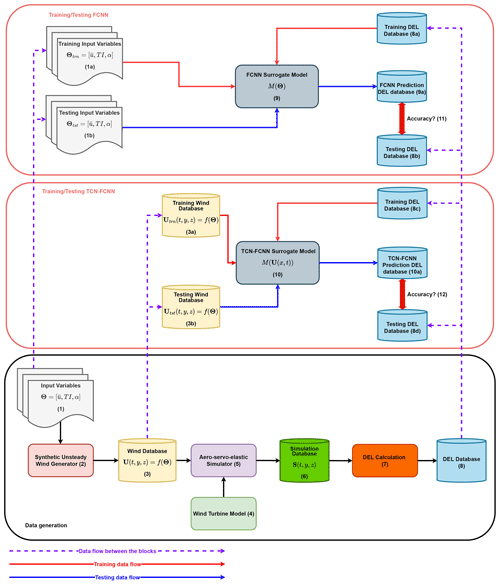
The presentation of the Methodology section in this paper has been adapted from the approach outlined in Schröder et al. (2020) due to its clarity and relevance to the current topic. The chosen framework is deemed to be an appropriate and effective means of conveying the necessary information in a concise and organized manner. The methodology used in this paper to map synthetic wind high-resolution time series to DELs is shown in Fig. 1. It involves developing a sequential ML model combined with FCNN architecture as the main SMs and utilizing a simpler FCNN for comparison purposes.

Figure 1 The data generation and SM training and testing methodology.

The configuration presented in Fig. 1 has three blocks. The bottom block is for data generation, which shows the procedure for building a database for the DEL from the input variables. The top two blocks are two methods used to build an SM from the generated data and input variables. The middle block presents the approach to building an SM that maps high-resolution wind time series to DELs based on TCN–FCNN architecture. The top block exhibits the process of creating an FCNN that projects the input variables onto the DEL (Dimitrov, 2019; Schröder et al., 2018). The larger frameworks and three blocks can be segmented into 12 smaller stages. Each step is summarized below. Throughout this paper, when we mention wind, we are specifically referring to unsteady wind.

• 1.

  Specify the input variable space, their distributions and boundaries, and afterwards, generate n samples X from the predefined variables. To enable tracking, every sample has been indexed. The database is split into two for training and testing:

  • 1a.

    Training input variables. These include 90 % of the samples randomly selected. Therefore, the size of this database is 0.9 n. The indices of the randomly selected samples idx_input have been stored.

  • 1b.

    Testing input variables. These include the remaining 10 % of the samples. As a result, the size of this database is 0.1 n.

• 2.

  The n generated samples are the inputs to a wind generator. Each sample from the input variable space generates one synthetic wind time series with the length of t time steps.

• 3.

  The n synthetic wind time series are stored in the wind database. The database size is n×t, where t is the number of time steps in the time series. For training/testing purposes, this database is split into two parts:

  • 3a.

    Training wind database. This includes 90 % of the main synthetic wind time series database randomly selected. Consequently, the size of this database is 0.9n×t. The indices of the randomly selected samples idx_wind have been stored.

  • 3b.

    Testing wind database. This includes the remaining 10 % of the main synthetic wind time series database. The size of this database is 0.1n×t.

• 4.

  The wind turbine model is an input to the aero-servo-elastic simulator. The model comprises three modules: aerodynamic, controller and aeroelastic.

• 5.

  The aero-servo-elastic simulator is a time-marching solver that takes synthetic wind time series and the wind turbine model as the inputs and delivers force, moment and load time series at l wind turbine components as the outputs.

• 6.

  All the n outputs of the previous step's simulations are stored in a database. In the simulation database, each simulation includes the l wind turbine component load time series for t time steps for one sample from the input variable space. Therefore, the database size is $n\times m\times t$.

• 7.

  The time series output is analyzed to determine the DEL of the loads on the l wind turbine components.

• 8.

  For every wind turbine component in the DEL database, each simulation output yields a single DEL data point. Therefore, the database size is n×l. Every row in the DEL database has an index that corresponds to the index of its input variable sample. As we train two SMs with the database, we split the database into training and testing databases twice. Thus, there appears to be an overlap between the testing and training databases. However, as we have utilized them to train and test two distinct SMs, we do not anticipate any issues arising from this situation.

  • 8a.

    Training DEL database members are selected based on the idx_input indices. Therefore, this database includes 90 % of the DEL, and the size is 0.9n×l.

  • 8b.

    The testing DEL database includes the remaining 10 % of the members of the DEL databases. Hence, this database size is 0.1n×l.

  • 8c.

    Training DEL database members are selected based on the idx_wind indices. Therefore, this database includes 90 % of the DEL, and the size is 0.9n×l. As mentioned before, there is an overlap between this database and the database in 8a.

  • 8d.

    The testing DEL database includes the remaining 10 % of the members of the DEL databases. Correspondingly, this database size is 0.1n×l.

• 9.

  The SM with FCNN composition trains and validates using the database in 3a as the input and the one in 8c as the output.

  • 9a.

    For testing, the trained FCNN SM takes the database in 3b as the input and provides FCNN prediction DEL as the output.

• 10

  The SM with TCN–FCNN architecture trains and validates using the database in 3a as the input and the one in 8c as the output.

  • 10a.

    For testing, the trained TCN–FCNN SM takes the database in 3b as the input and provides TCN prediction DEL as the output.

• 11.

  By comparing 9a with 8b, one can determine the accuracy of the trained FCNN SM.

• 12.

  By comparing 10a with 8d, one can determine the accuracy of the trained TCN–FCNN SM.

The aim of building and training a simple FCNN SM is to compare its accuracy and performance with those of the TCN–FCNN SM. The FCNN SM is not the ground truth in this work; however, it has proven to provide acceptable accuracy for a similar input variable space (Dimitrov, 2019; Schröder et al., 2018).

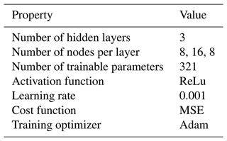
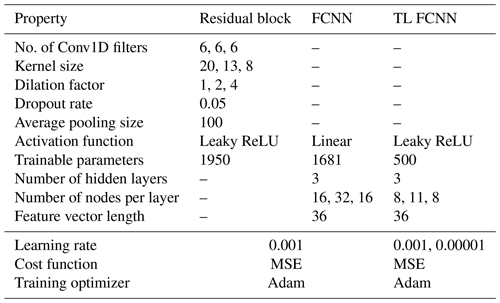
After building and training the TCN–FCNN, we show its versatility by examining the SMs with a synthetic wind including wake time series input. In other words, we test the SMs for a turbine in the downstream wake of another turbine. We developed smaller synthetic wind time series databases with wake effects, simulation outputs and their DELs. Moreover, we use TL to improve the SMs' performance over the wake. The architecture details for FCNN and TCN–FCNN provided in Tables 1 and 2 are experimentally obtained.

Table 1 FCNN architecture details.

Table 2 TCN–FCNN architecture properties and details for both the main approach and the TL approach. The TL approach is introduced in Sect. 2.6. TL FCNN learning rates are for the initial training and subsequent fine-tuning.

2.1 Fully connected neural network surrogate model

After preparing the DEL database, we can begin training the SMs. The primary objective for the SMs is to map the input space to the output. Various mapping and regression methods are available for this task, but we suggest utilizing data-driven ML methods due to their ease of use and versatility. We developed two SM architectures: an FCNN and a TCN–FCNN. Here, the FCNN is a simple three-layer feed-forward ANN. The feed-forward ANNs are well studied and explained in the literature. For further explanation, we recommend referring to Goodfellow et al. (2016).

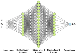
In order to train the FCNN, the input variable sample database is randomly divided into two parts: a training set comprising 90 % of the samples and a testing set comprising 10 % of the samples. These samples are uniquely indexed, and the training and testing set indices are stored and tracked. The DEL database is similarly divided into training and testing sets, using the same indices as the input samples. To prevent data leakage, we ensure that there is no overlap between the training and testing databases. Once the training and testing databases are prepared, the FCNN is trained using the input variable space samples as input and the DEL as output. The trained network is then tested using the testing input variable database to generate the prediction DEL. Finally, we compare the prediction DEL with the testing DEL to measure accuracy. By following this process, we can ensure that the FCNN is accurately trained and tested, producing reliable results. Figure 2 shows the implemented network architecture. The input layer receives three input variables in the FCNN, while the output layer is responsible for the DEL. The weights on each neuron are determined through the training process using the weight optimizer. After the training, the FCNN is ready to predict the output based on the unseen (testing) data. Table 1 presents the FCNN model details.

Figure 2 Architecture of the FCNN with three hidden layers. The number of nodes represents the implemented architecture.

2.2 Temporal convolutional network–fully connected neural network surrogate model

In this section, we explain the TCN–FCNN architecture that we used to build an SM. Firstly, we provide an overview of the key components that make up a TCN. We demonstrate how it can be effectively combined with an FCNN.

The TCN is a novel approach that utilizes the benefits of a one-dimensional convolutional neural network to perform sequential modelling (Bai et al., 2018). Sequential modelling can be defined as a tool to map a sequential input x₀, x₁, x₂, … ,x_n to a sequential output y₀, y₁, y₂, … ,y_n as shown in Eq. (1).

$$\begin{array}{}\text{(1)}& \widehat{y_{\mathrm{0}}},\mathrm{\dots },\widehat{y_n}=f\left(x_{\mathrm{0}},\mathrm{\dots },\widehat{x_n}\right)\end{array}$$

The TCN is a member of the convolutional neural network (CNN) family. CNNs have been used and are well known for classification purposes (Long et al., 2015). CNNs' basics are well studied in the literature, and the interested reader is referred to Goodfellow et al. (2016) and Long et al. (2015). Research has shown that the TCN is better than the recurrent neural network (RNN) and LSTM in terms of performance, implementation, flexibility and versatility (Fawaz et al., 2019; Bai et al., 2018). In this work, we only employ the TCN for regression purposes. The TCN is based on three main concepts: (a) the length of the output and input is the same, and (b) data should not leak from the past to the future. In other words, the value of each data sequence in the output only depends on the past data sequences in the input, and (c) it needs to be applicable to a long data sequence. To tackle these, one can use the following techniques (Bai et al., 2018):

• a.

  The TCN employs a one-dimensional CNN architecture, wherein each hidden layer is of the same length as the input layer. To ensure consistent length, zero padding is incorporated in successive layers.

• b.

  In order to avoid data leakage, TCN utilizes causal convolution architecture. In causal convolutions, the sequence n of the output solely relies on the sequences proceeding sequence n in the prior layer.

• c.

  For the simple causal convolutions, the length of the sequences that it can capture is a multiplication of the network depth. It makes the model deep and computationally demanding for long sequential data with vanishing gradients. The solution to this challenge is to utilize dilated convolution. By using dilated convolution, the network is able to increase its receptive field significantly in an exponential manner. For a one-dimensional sequential input x, a filter f and the element s of the sequence, one can define the operation F as

  $$\begin{array}{}\text{(2)}& F\left(s\right)=\left(\mathit{x}{\ast }_{d}f\right)\left(s\right)=\sum _{i=\mathrm{0}}^{k-\mathrm{1}}f\left(i\right)\cdot {\mathit{x}}_{s-d\cdot i},\end{array}$$

  where ∗ is the convolution operator, d is the dilation factor, k is the kernel size and $s-d\cdot i$ points out the direction of the past. In dilated convolution, the dilation factor increases exponentially with the level of the network depth. Figure 3a shows an illustration of a dilated convolution. The history of the sequences that a layer can take into account is (k−1)d.

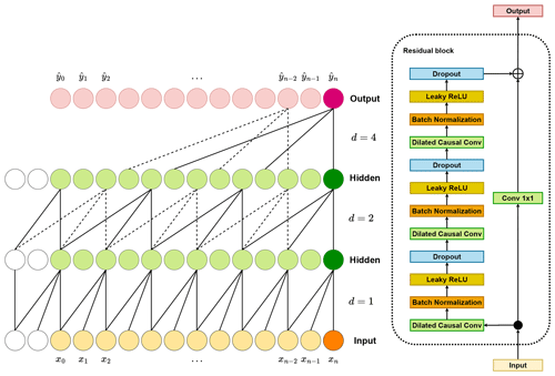
Figure 3 (a) Illustration of a dilated causal convolution example, with kernel size k=3 and dilation factors $d=\mathrm{1},\mathrm{2},\mathrm{4}$. The receptive field has the ability to encompass all values present within the input sequence. The white circles show the zero padding in the layers. (b) Dilated causal CNN and the residual block for the TCN.

As the TCN needs to take into account larger sequential data, it needs many layers and, as a result, gets deep quickly. This causes the network's problem of performance degradation, which needs to be stabilized. Therefore, we utilize a residual block as a replacement for a convolutional layer (Bai et al., 2018; He et al., 2015). The residual block methodology incorporates a branching mechanism where the input is injected into the output, passing through a CNN. The residual block used in this study is shown in Fig. 3b.

For this study, we utilized the aforementioned TCN to extract features from the input time series. Feature learning or feature extraction is the process by which the machine learning model converts the raw data into an “internal representation”, feature vector or latent space (LeCun et al., 2015). Then this feature vector is employed to detect the output pattern through a secondary machine learning subsystem. In this study, we took advantage of the TCN's ability to extract features in the sequential data. Thereafter, we used the features as the input to an FCNN. The integration of the TCN and FCNN enabled us to map the wind time series into DEL. Westermann et al. (2020) used a similar approach but for a different application. The explained technique is illustrated in Fig. 4. The residual block in Fig. 4 is made up of the components depicted in Fig. 3b. The definition of each block is beyond the scope of this work. For a comprehensive understanding, readers are encouraged to refer to Goodfellow et al. (2016).

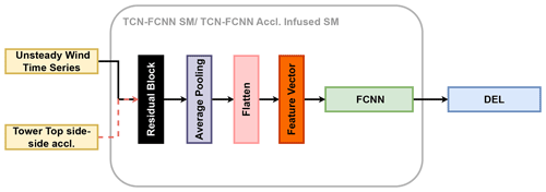
Figure 4 The TCN–FCNN architecture. The tower top side–side acceleration is an optional input that we discuss further in Sect. 4.1.

With all the requisite SM components in place, we can proceed with the training and testing phases. As mentioned before, we indexed the samples, and TurbSim generated wind time series outputs. In the same manner as explained in Sect. 2.1, the synthetic wind time series database is divided into training and testing databases, where 90 % of the database is selected for the training, and the remaining 10 % goes for testing. This means 90 % of the full 600 s wind time series is selected for training, and 10 % of the full 600 s wind time series is used for testing. We maintain the same training–testing division of the datasets as in Sect. 2.1 to simplify the comparison of testing results between FCNN and TCN–FCNN. As the indices for the training and testing databases are known, they are used to divide the DEL database into training and testing databases. With the training and testing databases ready, the TCN–FCNN is trained on the training data. Afterwards, we utilized the trained model to forecast DEL using the synthetic wind time series that was not included in the training database. The predicted DEL is then compared with the testing DEL to measure the accuracy of the mapping. The specifications of the TCN–FCNN SM employed are detailed in Table 2.

2.3 Variable input space boundaries, distributions and sampling

For the data generation, selecting the appropriate input variable space, the boundaries for each variable and their distributions is crucial. Depending on the problem at hand, different input variables might be needed. As we only considered one onshore wind turbine in this study, only the input variables that affect the wind generation are considered. These three variables are mean wind speed $\overline{u}$, turbulence intensity TI and wind shear α. Therefore, the input space Θ can be defined as

$$\begin{array}{}\text{(3)}& \mathrm{\Theta }=(\stackrel{\mathrm{‾}}{u},\mathrm{TI},\mathit{\alpha }).\end{array}$$

The boundaries and distributions of our input variables help define the conditions for which our models are designed. It is important to note that wind speed is considered an independent variable, while the other two variables' boundaries and distributions depend on the wind speed. We have selected the variables, their boundaries and their distributions to build the database based on research presented in Dimitrov (2019). Our use of the QMC Sobol sampling method (Sobol', 1967) allows for accurate sampling of the predefined joint distributions in a deterministic non-repetitive manner. In this study, the Sobol sampling method is preferred as it is consistent and computationally efficient (Kucherenko et al., 2015). Moreover, this sampling method is reproducible and provides better uniformity properties of the samples over the distributions (Renardy et al., 2021). In the following, when we refer to the sample, it means a vector of three elements, namely mean wind speed, turbulence intensity and wind shear.

2.4 Simulation and damage equivalent load database creation

The samples from the input variable space are the inputs to the synthetic wind generator. Each sample from the space provides one input to the generator. The output of the generator is a “full-field” synthetic wind time series (Jonkman, 2009). The synthetic wind generation basics are explained in length in Veers (1988). In this study, we employed TurbSim to generate the synthetic wind fields (Jonkman, 2009). From each sample, the three input variables ($\stackrel{\mathrm{‾}}{u}$, TI, α) are directly taken into the TurbSim input file and generate one synthetic wind time series using TurbSim. To guarantee that every time series created is distinct, a unique seed number is assigned to each sample. The output of the wind generator can be defined as a function of the sample:

$$\begin{array}{}\text{(4)}& U(t,y,z)=f\left(\mathrm{\Theta }\right).\end{array}$$

The output has spatial and temporal components $U(t,y,z)$. The spatial component of the full-field synthetic wind comes from the grid points, which are defined over the wind turbine rotor plane. The output of TurbSim provides one time series of synthetic wind at each grid point in x, y and z directions, namely u, v and w. These time series are correlated to each other, depending on the mean wind speed and their distance from each other (Veers, 1988; Jonkman, 2009).

The full-field synthetic wind is the input to the aero-servo-elastic simulations. To run these simulations next to the synthetic wind time series, the aerodynamic model, aeroelastic model and controller model are required too. This study used an onshore model of the NREL 5 MW reference wind turbine (Jonkman et al., 2009). The wind turbine model includes aerodynamic, aeroelastic and controller submodules. To run the simulations, we used OpenFAST, the time-marching aero-servo-elastic solver developed by NREL (Jonkman et al., 2022). OpenFAST's output includes both temporal and spatial dimensions, with loads provided from various wind turbine components located at different positions, such as blades, towers and gearboxes. This spatial aspect is integral to understanding the full scope of the data. The simulations in this study follow the IEC standards for power production design load case (DLC) 1.2, as stated in IEC standards (International Electrotechnical Commission, 2019).

Thus far, we have established a database that comprehensively incorporates all the simulation output time series data. Once we have that, the data are processed to obtain the simulation time length statistics and DEL for evaluating the loads and fatigue. DEL calculation is based on the Palmgren–Miner linear damage rule as explained well in Thomsen (1998) and Stiesdal (1992). DEL can be formulated as

$$\begin{array}{}\text{(5)}& \mathrm{DEL}={\left({\displaystyle \frac{\mathrm{\Sigma }{n}_i{R}_i^m}{n_{\mathrm{eq}}}}\right)}^{\mathrm{1}/m}.\end{array}$$

In the given context, m represents the Wöhler exponent, while R_i and n_i correspond to load ranges and the respective number of cycles. The output is obtained through rain flow counting of the load time series (Thomsen, 1998). Here, n_eq is the equivalent number of load cycles. For our scenario, the simulation duration is 600 s with a frequency of 1 Hz, resulting in n_eq=600. This means the DELs are based on 600 s time series. The DEL database includes all the calculated DELs from every simulation at its outputs.

2.5 Simplified wake model

Once the SMs are built and trained, we assess their versatility by testing them with a turbine in the wake. To proceed, we must create a new database that includes the synthetic wind and DEL with consideration given to wake effects.

The wake caused by a wind turbine has been studied extensively and is out of this paper's scope. Different methods and models exist to implement wakes in the aerodynamic simulation of a wind turbine (Sanderse et al., 2011; Göçmen et al., 2016). For the sake of simplicity and ease of implementation, we limit the study to a simplified wake definition, with the study turbine in the wake of one turbine only. The simplified wake includes a non-uniform wind speed deficit and an increase in turbulence intensity across the rotor. To implement wakes in the synthetic wind time series, we used the method explained in William et al. (2022).

For the velocity deficit caused by the wake over the rotor plane, we utilized the super-Gaussian deficit (Blondel and Cathelain, 2020). We used the formulation developed by Ishihara and Qian (2018) for the added turbulence intensity model. Moreover, similar to Bastankhah and Porté-Agel (2014) and Ishihara and Qian (2018), we assume the linear expansion of the wake that occurs downstream of a turbine. The following are the steps we took to implement the downstream simplified wake model:

1. Using the Sobol sampling method, take 2ⁿ samples from the input variables ($\stackrel{\mathrm{‾}}{u}$, TI, α), as explained in Sect. 2.3.

2. Knowing the turbine thrust coefficient C_t at each wind speed, the ambient turbulence of the freestream and the distance between the turbines, one can calculate the downstream wake width based on the formulation in Ishihara and Qian (2018).

3. With wake width calculated in the previous step, one can calculate the velocity deficit (William et al., 2022; Blondel and Cathelain, 2020) and added turbulence intensity (Ishihara and Qian, 2018).

4. Both calculated velocity deficit and added turbulence intensity have spatial distribution over the rotor plane. We considered this distribution by modifying the mean wind speed and turbulence intensity of the samples for the first step. For the added turbulence intensity, the average over the rotor disk is added to the TI value of the sample. For the deficit wind velocity, the harmonic mean over the rotor disk is deducted from the sample mean wind speed $\stackrel{\mathrm{‾}}{u}$ (William et al., 2022).

5. With the modified Sobol samples in our possession, we used TurbSim to generate synthetic wind time series from each modified sample. Remember that these synthetic wind time series have modified turbulence intensity and reduced mean wind speed, but the Gaussian deficit has not yet been included.

6. For the generated synthetic wind by TurbSim, for the mean wind speed of $\overline{u}$, the wind speed in time t at each (y, z) point can be defined as

   $$\begin{array}{}\text{(6)}& U(t,y,z)=\stackrel{\mathrm{‾}}{u}(y,z)+\stackrel{\mathrm{̃}}{u}(t,y,z),\end{array}$$

   where $\stackrel{\mathrm{̃}}{u}(t,y,z)$ is the 0 mean turbulence, and $\stackrel{\mathrm{‾}}{u}(y,z)$ is the constant mean wind speed over the rotor plane. The inclusion of the velocity deficit caused by the wake in the generated synthetic wind can be expressed as

   $$\begin{array}{}\text{(7)}& U^{*}(t,y,z)=\mathit{\varphi }(y,z)+\stackrel{\mathrm{̃}}{u}(t,y,z),\end{array}$$

   where $U^{*}(t,y,z)$ is the modified wind field, and ϕ(y,z) is the velocity deficit distribution over the rotor y–z plane, which we calculated in Eq. 3.

We use synthetic wind with a velocity deficit and added turbulence intensity to run OpenFast simulations containing the simplified wake model and calculate the DEL as described in Sect. 2.4.

2.6 Transfer learning

According to Goodfellow et al. (2016), transfer learning aims to utilize what has been learned in one context to improve the “generalization” in another context. For this study, we use TL for the cases with a wake to improve their prediction.

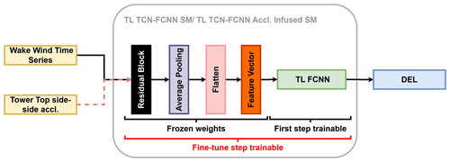
After following the steps outlined at the beginning of this section, we obtain trained SMs that are able to accurately predict the DEL of wind turbine components under freestream synthetic wind conditions. We then use these models to predict DEL in the wake of a turbine. We implement TL to enhance our predictions by loading the trained SMs and freezing their weights, making them untrainable. Then, we remove the FCNN part of the TCN–FCNN and replace it with a trainable FCNN. The new FCNN system we are using now has a simpler architecture compared to the one we previously used for training and testing on the freestream data. Essentially, we now have a frozen-weight (untrainable) TCN along with a trainable FCNN. As with the previous training process, we utilize 90 % of the wake databases for training and 10 % for testing. The training has two steps: the first step is to train the aforementioned combination of the untrainable TCN and trainable FCNN to the desired accuracy, and then fine-tune the TL model by unfreezing the TCN part weights and training them on the same data again but this time with a smaller learning rate. The properties and details of the TL FCNN are shown in Table 2. Figure 5 illustrates the architecture used for the TL.

Figure 5 The frozen TCN with a trainable simple FCNN for the first step of TL, the fine-tuning step.

2.7 Training–testing

Now that we have constructed all the necessary databases, we can begin the training process. We must first normalize the data before training the SMs. In this study, we employ min–max scaling for both input and output values, scaling them to a range of 0 to 1. The input variables are scaled individually, while all the synthetic wind time series, regardless of the mean wind speed, are included in a single scaling procedure. During the training process of the TCN–FCNN and FCNN models, we implemented a separate scaling of the DEL of each output channel. This approach was necessary to ensure the scaling was tailored to the specific needs of each channel. A total of 12 SMs were trained, with 6 models being trained for each respective network architecture type.

Table 3 Training settings for the SMs.

The total number of samples in the dataset is 32 768. As mentioned in Sect. 2.2, this dataset is randomly split into two parts for different purposes by choosing the indices of the samples through a non-repetitive random number generator. The training set contains 90 % of the samples, and the testing set contains 10 % of the samples. When randomly selecting data for testing and training, it is essential to be mindful of potential data leakage, particularly when working with measurement time series data. In our specific scenario, data leakage is not a concern as the simulated data samples are statistically independent and turbulence seeds are unique. Instead of training the SMs on the entire training data at once, the training dataset is divided into batches of 256 samples and then trained on those batches. The SMs are trained on each batch, and after going through all the batches of the training dataset, one “epoch” is completed. The main optimizer employed in the SM training in this work is Adam (Kingma and Ba, 2017). Taking all the training datasets for the training while employing Adam requires a large amount of memory, and the optimizer may lead you to a “saddle point” (Ge et al., 2015). One can tackle both of these issues in training by dividing the training data into batches, as explained before. One disadvantage of this method is that it requires more epochs for the model weights to be fully trained and converged.

In this study, we used Python package tensorflow for the ML model development, training and testing (Abadi et al., 2024). An outline of the settings and details for training in tensorflow can be found in Table 3.

We employed early stopping for the training as it reduces the required training time. Once the training phase is complete, the remaining 10 % of the data that were not used during training are utilized for testing purposes. The output of the testing procedure provides the accuracy of the fitted models. For this study, we use the coefficient of determination, R², and NRMSE as the measures for the fitted models' accuracy.

3 Data generation

This section presents the procedure, conditions and assumptions for data generation and management.

3.1 Input variable boundaries, distributions and sampling

To generate the synthetic wind time series and DEL, we used the input variable space, as explained in Sect. 2.3. The mean wind speed is sampled from a uniform distribution, where the boundaries are decided based on the NREL 5 MW wind turbine characteristics between the cut-in and cut-out wind speed (Jonkman et al., 2009). For every wind speed sample, we took a sample from the TI and α too. The other two input variables are also defined as a uniform distribution, whose boundaries are a wind speed function. For the TI, the boundaries are based on the IEC class 1A values (International Electrotechnical Commission, 2019). We choose the same boundaries for wind shear α as Dimitrov (2019). The input variables and their boundaries can be found in Table 4.

Table 4 The input variable boundaries.

Here, (1) is from IEC class 1A, I_ref=18 %; (b) ${\mathit{\alpha }}_{\mathrm{ref},\mathrm{LB}}=\mathrm{0.15}$ and ${\mathit{\alpha }}_{\mathrm{ref},\mathrm{UB}}=\mathrm{0.22}$ are reference wind shear at 15 m s⁻¹; (c) ${\stackrel{\mathrm{‾}}{u}}_{\max }=\mathrm{25}$ m s⁻¹ is the upper bound of the wind speed; and (d) R is the rotor radius, and z is the hub height.

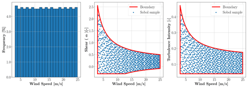
Figure 6 A total of 1024 Sobol samples from the predefined distributions for $\stackrel{\mathrm{‾}}{u}$, TI and α with the boundaries of the variables.

Once we have established the joint distributions and boundaries, we can generate sample points for the input variable space. As described in Sect. 2.3, we used the Sobol sampling method for this study. The Sobol samples need to be of the order of 2ⁿ, otherwise they lose their balance properties (Owen, 2021). Therefore, we took n=2¹⁵ samples from the predefined distributions. We decided to have a conservative number of samples, as the Sobol sampling method enables us to reduce the number of samples without losing the benefits of the method or resampling the domains. To generate an example of the variable space, we took 2¹⁰=1024 samples from the predefined distribution in Table 4. The samples and the input variable boundaries are displayed in Fig. 6.

3.2 TurbSim and OpenFAST output

As mentioned before, we use each sample from the input variables to generate a unique synthetic wind time series using TurbSim. Every TurbSim output generated from each sample is assigned a unique seed number to ensure no repeating seeds. The TurbSim output format is well described in Jonkman (2009). We acknowledge that the seed number influences the DEL values as indicated by Liew and Larsen (2022). Nevertheless, utilizing Sobol sampling allows the TI values to emulate the variability in wind time series resulting from different seed numbers. Furthermore, the training of the TCN–FCNN using actual input realizations, as opposed to solely relying on TI, is expected to mitigate the aforementioned issue significantly for the proposed method. In fact, if more seeds are required, the trained model could be utilized to make predictions on a broader spectrum of random seeds. For this study, we used a 15 by 15 grid over the rotor's plane to build the database. However, for training and testing, only 9 out of 225 points on the rotor plane, as depicted in Fig. 7a, were considered. For these nine points on the rotor plane we only take into account the wind in the x direction. Our tests show including the wind in the y and z directions would not improve the training or testing results; therefore, they are omitted. These nine synthetic wind time series are approximately located at the middle of the rotor and hub height. The number of points on the rotor plane was determined experimentally. This decision was guided by the minimum requisite wind time series data from the rotor plane, which facilitated the training of an accurate model. In general, adding more input features to the SMs increases the number of training parameters and training complexity without yielding additional benefits. This would increase the training dataset requirement to mitigate issues such as overfitting and non-convergence. In terms of real-world application, with nine points, it could be considered for use in scenarios such as field light detection and ranging (lidar) measurements. Our tests show other configurations of the points (e.g. circular layout of points) have little impact on the results. The grid points are selected to be roughly located at the blades' mid-span. This selection is illustrated in Fig. 7a. Regarding the time component, the synthetic wind time series has a frequency of 20 Hz, with a duration of 720 s. After running the simulation and later in the training/testing step, we upsample the synthetic wind to 1 Hz due to the hardware constraint.

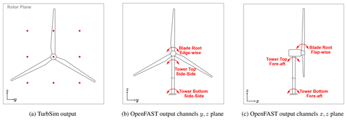
Figure 7 (a) Illustration of selected TurbSim output grid point locations as the input to the SM for training and testing. Panels (b) and (c) show a schematic drawing of a turbine, with the output load channels.

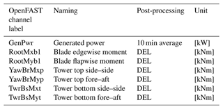
As mentioned, we run aeroelastic simulations on an onshore NREL 5 MW model using OpenFAST. OpenFAST can provide an extensive set of outputs, namely channels, at different components of the turbine. The channels and their descriptions can be found in Jonkman and Buhl (2005). For this study, we took into account six-moment output channels and the average generated power for the training/testing objectives. These six moments are blade root edgewise and flapwise moments, tower top fore–aft and side–side moments, and tower bottom fore–aft and side–side moments. Figure 7b and c illustrate a schematic drawing of the wind turbine with the load channel locations that we used for training/testing in this study. The OpenFAST output channel label and its corresponding naming for this study are provided in Table 5.

Table 5 Channel label, naming and units.

We run $n={\mathrm{2}}^{\mathrm{15}}=\mathrm{32}\mathrm{768}$ aeroelastic simulations using OpenFAST for this study. We run the simulations in 2048 batches of 16 simulations in parallel using Digital Research Alliance of Canada resources. Each simulation ran for 720 s, but the first 120 s of the simulation output was discarded to avoid any initialization effect. The time step for the aeroelastic simulation was set to 0.00625 s, while the output resolution is 20 Hz. After running all the simulations and building the simulation output database, we calculate the DEL for each simulation, for the interested output channels for Wöhler exponent m=4 and n_eq=600 in Eq. (5), as mentioned in Sect. 2.4. Moreover, we considered the 10 min average of the generated power. To read the OpenFAST output files and calculate the DEL, we used the Python pyfast library (Branlard, 2023).

3.3 Turbine in wake output

Our aim is to test the effectiveness of the trained TCN–FCNN SMs by using wake input and specifically to determine if the model, which is trained on a turbine in the freestream, can accurately predict the DEL of a turbine in a wake as well. The test scenario involves one turbine in the freestream, which the SMs are trained on, and one turbine in the downstream wake. The distance between the two turbines is 7 D, where D represents the rotor diameter. In our specific case, we consider the rotor diameter of 126 m for NREL 5 MW, which results in a distance of 882 m between the two turbines.

We followed the same process described in Sect. 3.1 by taking 2048 samples from the distributions outlined in Table 4. To calculate the wind velocity deficit and add turbulence, we used the Gaussian model (Blondel and Cathelain, 2020; Ishihara and Qian, 2018), as explained in Sect. 2.5. We then adjusted the $\stackrel{\mathrm{‾}}{u}$ and TI of each sample based on the harmonic mean of the wind velocity deficit and the arithmetic mean of the added turbulence intensity over the rotor. Using the modified samples, we generated 2048 TurbSim full-field outputs, following the process explained in Sect. 3.2. With the TurbSim output now available with modified $\stackrel{\mathrm{‾}}{u}$ and TI, we utilized a Python script to offset the generated synthetic wind with the Gaussian velocity deficit profile (William et al., 2022).

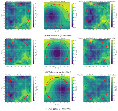
Figure 8 The velocity deficit implementation on a TurbSim output with the added turbulence intensity.

In Sect. 2.5, it is explained that the wind velocity deficit has a distribution across the y–z plane. This distribution can shift across the rotor plane depending on the location of the wake centre. We established three wake cases with wake centres located at −30 and 90 m, 0 and 90 m, and 30 and 90 m on the y–z rotor plane. The wake centre is assumed not to move vertically since both turbines have the same hub height of 90 m. Figure 8 illustrates an example of the velocity deficit effect on the TurbSim output. In Fig. 8, the first column shows the TurbSim output with the added turbulence intensity, the middle column is the Gaussian velocity deficit for the aforementioned wake centres and the last column is the first column with the velocity deficit offset. They are all a snapshot of the TurbSim output at 320 s, and the input samples are $\stackrel{\mathrm{‾}}{u}=\mathrm{13.42}$ m s⁻¹, TI=11 % and α=0.107. The red circle is the rotor disk.

As all the 2048 TurbSim outputs are at hand, one can run OpenFast simulations and calculate DEL as explained in Sect. 3.2.

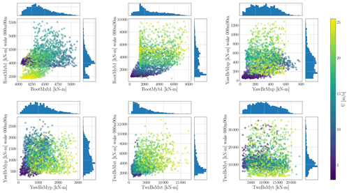
To better understand the changes in DEL when the turbine is in wake conditions versus freestream, we present the raw DEL for both scenarios in Fig. 9. This plot compares all 2048 samples when the wake centre is at 0 and 90 m with the corresponding Sobol samples from the freestream for all six channels in the scatter plots and their corresponding histograms. The figure illustrates a shift in the DEL values and their distribution when the turbine operates in the wake of another turbine.

Figure 9 Raw DEL from both freestream and wake databases for 2048 samples. The colour map represents a range of changes in the mean wind speed of the samples.

4 Results and discussion

To this point, we explain the background methods used in this work. This section delivers and discusses the results.

4.1 TCN–FCNN results

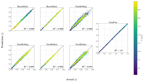
This section provides the output of the testing process, as explained before, for the TCN–FCNN SMs. Figure 10 shows the results of the testing on the trained SMs for each output-channel-scaled DEL. Each plot in the figure delivers one channel, and data connect to the mean wind speed of the samples using a colour map. Upon reviewing the outcomes, it is evident that the SMs offer precise prediction based on synthetic wind time series data that it has not previously encountered. Based on the colour maps, it is inconclusive to determine the correlation between the input variables of the sample and the accuracy of the fit.

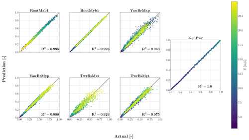
Figure 10 Testing results for TCN–FCNN trained SMs. The colour map represents a range of changes in the mean wind speed of the samples.

Although all channels have high R² values, the values decrease as we move from the blade root moments downwards. This decrease can be explained by the physical problem we are dealing with. The SMs have only one input, and they map wind input time series in the x direction to DEL outputs. The loads closer to the rotor are more affected by the wind input, while the structural dynamics of the wind turbine influence the further loads. Both fore–aft and side–side moments exhibit similar behaviour, but fore–aft moments are predicted more accurately. Therefore, it is reasonable to assert that the fore–aft moments are predominantly attributable to the wind, whereas the structural dynamics more significantly influence the side-to-side moments. To test this hypothesis, we infused the input of the TCN–FCNN with the tower top side–side time series acceleration a_TTy. In other words, the TCN–FCNN maps the combination of synthetic wind time series and tower top side–side acceleration time series to DEL. Figure 4 visually represents this network with tower top side–side acceleration as an optional input.

The modified SMs used for this are identical to those shown in Tables 2 and 3. The only difference is that the third dimension of the input shape in Table 3 has changed to 10 due to the concatenated time series. We followed the same process for training and testing these acceleration-enhanced SMs as we did for the original ones. In Fig. 11, the data indicate that incorporating the tower top acceleration time series into the input led to a better fit for the side–side moments, particularly for the tower bottom side–side moment. This confirms our hypothesis that these SMs can accurately capture the physics of the model at hand. One question that arises is why there is no improvement in the tower top side–side bending moment channel. The tower top side–side bending moment is primarily influenced by rotor torque rather than side–side acceleration. In contrast, the tower bottom side–side bending moment is caused by the side–side forces at the tower top, which are represented by the side–side acceleration. As a result, we do not see any improvement in the tower top side–side moment. One may argue that including the wind time series in the y direction in the input would improve the tower bottom side–side moment R² value. We tested this hypothesis, but it did not improve the accuracy of the TCN–FCNN model. For the sake of space, we do not include the results of this analysis here. However, the trained model and databases for this test are provided for the interested reader. Given that tower top acceleration cannot be obtained without direct measurement or conducting aeroelastic simulations, this SM is particularly suitable for virtual sensing (Moynihan et al., 2024) or DT applications, as mentioned in Sect. 1.

Figure 11 Testing results for TCN–FCNN trained SMs. The input for these SMs is infused with the tower top acceleration time series. The colour map represents a range of changes in the mean wind speed of the samples.

4.2 FCNN results

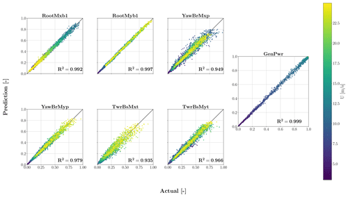
As mentioned in Sect. 2.7, we trained and tested the FCNN SM on the three input variable samples, namely wind speed, wind shear and turbulence intensity. The FCNN aims to map the three input variables to DEL. This is very similar to the approach that was employed in Schröder et al. (2020). The results are presented in Fig. 12. Similar to the TCN–FCNN results, the R² values decrease from the top to the bottom of the turbine. Considering the simplicity of the FCNN SMs, they perform very well in the testing phase.

Figure 12 Testing results of the FCNN on the trained SMs.

4.3 Result comparison

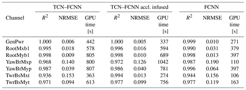
Up to this point, we trained three different types of SMs on our dataset. These SMs showed a good ability to predict the DEL from a limited amount of sequential data or input variable data. Each SM architecture has its own advantages and disadvantages. For TCN–FCNN architecture, the SMs can digest the complexities of wind time series. Nevertheless, the model is complex and loses accuracy for the channels that are not close to the rotor. On the other hand, FCNN architecture is simple and cheap to train, while it has higher R² values for the channels below the rotor. However, this model suffers from the same challenge in terms of R² value decline, and it is not prepared to take time series and needs input variables that may not be available all the time. For example, in reality, looking at what SCADA collects, the TI and wind shear are not necessarily available for all turbine types. To make the comparison more straightforward, the R² value for power and output channels and the required GPU time for the training are provided in Table 6.

Table 6 The accuracy of the fit and computational time for the SM training. NRMSE is in percentage.

The data presented in Table 6 reveal that all three SMs have consistently produced high R² values and a low NRMSE. Notably, the utilization of tower top acceleration as the added input to wind has significantly enhanced the accuracy of prediction for the tower bottom side–side moment. This improvement is a testament to the TCN–FCNN SMs' ability to comprehend the mechanics behind the input–output correlation. Regarding the computational cost, FCNN SMs are more efficient for all the outputs.

When examining Table 6, one might question the purpose of developing the TCN–FCNN SMs as they are more complex and computationally expensive. The TCN–FCNN approach offers a significant benefit by examining the wind's time series rather than solely its statistical properties. The DEL results from wind and/or wave time series oscillations. If we were to reduce these oscillations solely to wind or wave input statistics, this would undermine the precision, insight and perception of the DEL prediction. However, the TCN–FCNN can incorporate these oscillations and map them to the DEL. Similar approaches have led to similar outcomes, as shown in de N Santos et al. (2023), where the accuracy of the SM improved by incorporating the high-resolution time series as input.

Here, we calculate the DELs based on simulations lasting 600 s. However, in real-world scenarios, the data availability might be longer or shorter than 600 s. Therefore, one challenge here is to free the input from the time series' length, which is not within the scope of this study. We will explore the effect further in our future studies. We briefly discuss the shortening of the simulation length effect in Sect. 4.6.

We underline that the TCN–FCNN model can effectively decompose the wind field into its constituent features, which include the input variables. This capability was tested by expanding the feature vector in Fig. 4 with the three input variables. Even with this augmentation, the R² values remained consistent, reaffirming the robustness of the TCN–FCNN in characterizing the wind field. Essentially, a latent space has been identified by the TCN that is suitable for accurate DEL prediction by the FCNN stage.

We tested the TCN–FCNN architecture to assess its ability to handle ultimate loads. During our analysis, we found that the SMs could accurately predict ultimate loads with a comparable level of precision as DEL prediction. We do not include the results here for space efficiency, but the trained models and datasets are available for the interested reader.

4.4 TCN–FCNN SMs in wake with TL

Considering the methodology employed for incorporating wake effects into our simulations, the use of an FCNN proves ineffective in this context. The FCNN relies on input parameters such as mean wind speed $\stackrel{\mathrm{‾}}{u}$, turbulence intensity TI and wind shear α, which cannot adequately capture the complexities of wake interactions, as they cannot be condensed into a single scalar value. In a study by Dimitrov (2019), an FCNN-based surrogate model was utilized to model wake effects. It was noted that their model required additional inputs depending on the wind farm layout. In contrast, the TCN–FCNN approach, which relies solely on flow information at the turbine location, effectively addresses wake challenges without requiring additional inputs, assuming well-defined flow characteristics over the turbine. It is crucial to acknowledge the complexity of wake phenomena. Our claim is specifically about the SM's ability to accurately map a wake-distorted flow to DEL values, not to underestimate the intricacy of wake dynamics.

After training the TCN–FCNN and FCNN SMs, we tested the SMs on the input with the wake. The initial results without any TL did not provide an accurate prediction. Therefore, we used the TL as explained in Sects. 2.5 and 3.3. Table 3 details the training setting for the TL models. The training is done on 90 % of the turbine in wake databases, and testing is based on the remaining 10 %. We used both normal TCN–FCNN and acceleration-infused TCN–FCNN in the TL for the turbine in the wake. The results for three wake centres are presented in Table 7.

Table 7 The results for the turbine in wake SMs in predictions after going through two stages of TL. The TL is done on both TCN–FCNN and the acceleration-infused TCN–FCNN. For the sake of space, acceleration-infused TCN–FCNN is indicated as TCN–FCNN A.I. NRMSE is in percentage.

The results predicted in Table 7 follow a similar trend to those obtained from the freestream turbine for all three wake centres. However, the SMs infused with acceleration provide higher R² values for almost all cases compared to the freestream, where the effect was mainly limited to tower bottom channels. Since the turbine's behaviour is more complex in the wake, knowledge of its structural dynamics can be more influential in prediction. Therefore, including a channel from the turbine structure can aid the SMs in training a more accurate model and providing better predictions. It is worth noting that this training is conducted on only 1844 out of 2048 data points in the wake database, which is relatively small. Despite this, the model's ability to have a low NRMSE and high R² values demonstrates its strength.

4.5 How much data are enough data?

One question that needs to be answered is how much data are enough to train these SMs accurately. In other words, we need to determine if reducing the number of sample points will affect the accuracy of the predictions made by the SMs. As we used the QMC method for sampling in this study, we can easily decrease the number of samples without having to redo the simulations. However, as our samples are based on Sobol samples, we need to stick to the 2ⁿ rule. To determine the amount of data needed, we trained the SMs on a smaller number of samples ranging from 2⁶ to 2¹⁴. Then, we randomly selected 1000 samples from the remaining input samples for prediction. For example, in the case of 2¹⁰, we trained the SMs on 1024 Sobol sample data points and randomly selected 1000 samples from the remaining 2¹⁵–2¹⁰ samples for prediction. This enabled us to ensure fairness in comparing the R² values without any data leakage. The sensitivity analysis results in Fig. 13 indicate that the R² value remains relatively high across all channels until the number of samples is reduced to 2⁸.

Figure 13 Sensitivity of R² to the number of training samples. The y axis is on a logarithmic scale with a base of 10, while the x axis is on a logarithmic scale with a base of 2.

This shows that the SMs are versatile and do not require many sample points to make accurate predictions. The versatility of the SMs can be attributed to the simplicity and power of the models for providing accurate predictions and the effectiveness of Sobol sampling in covering the input variable domains even with a low number of data points. This coverage helps the SMs to interpolate well between the data they are not trained on. The displayed data in Fig. 13 indicate that FCNN SMs exhibit less sensitivity to the number of samples. This observation aligns with the expectation that FCNN SMs possess a simpler architecture and fewer parameters to be trained. Therefore, the trained model improvement is minimal after passing the threshold of the number of samples. In the TCN–FCNN SMs, the improvement of the R² value varies depending on the channel. The tower channels exhibit a greater rate of R² improvement as compared to the rotor channels, with the side–side moment channels of the tower being the most prominent example. Additionally, acceleration-infused TCN–FCNN shows higher improvement rates for tower top side–side and tower bottom fore–aft channels.

4.6 Time series length and data augmentation

In this study, we used a 10 min time series for both input and output of the OpenFAST simulation. This is a common practice in the wind turbine engineering field as recommended by standards (International Electrotechnical Commission, 2019). Yet, from the perspective of lidar and a wind turbine controller, a 10 min time series may be relatively long. Therefore, we aimed to include the ability to handle shorter synthetic wind time series and map them to DEL, which would be more attractive. Besides, in the field of machine learning, having enough training data is a challenge, and data augmentation is a solution (Mikołajczyk and Grochowski, 2018). To satisfy these two purposes, we attempted to augment data by dividing the 600 s synthetic wind and load time series into shorter segments and calculating DEL from those segments. If possible, the goal was to use even less than the minimum required number of simulations. However, our investigations have revealed that subsampling the 600 s load time series into segments shorter than 300 s adversely affects the accuracy of the DEL calculation. This is due to missed cycle counting of the shorter data length obtained from OpenFAST output. Hence, this approach was not included in this paper.

5 Conclusion

This study explores the potential of employing a sequential ML model to develop an SM that correlates high-resolution wind time series with the DEL of wind turbine components. The methodology utilized in this paper involves creating TCN–FCNN architecture for mapping synthetic wind time series to DEL, alongside a simpler FCNN for comparative purposes. We divided our methodology into 12 stages, including specifying the input variable space, generating synthetic wind time series, conducting aero-servo-elastic simulations, calculating DEL, splitting the data into training and testing databases, and building SMs. Additionally, we build a database of synthetic wind time series and DEL for a turbine in a wake to test the versatility of the TCN–FCNN SMs using TL.

Our work begins with defining the input variable space and determining their boundaries, distributions and sampling methods. We use a QMC Sobol sampling technique to generate non-repetitive samples, guaranteeing uniformity, traceability and reproducibility. Next, we continue with the generation of synthetic wind time series using TurbSim, based on the input variable samples. These time series are stored in the wind database, forming the basis for subsequent simulations. The aero-servo-elastic simulations are performed using the NREL 5 MW reference wind turbine model and OpenFAST, following IEC standards for power production DLC 1.2 (International Electrotechnical Commission, 2019). The simulation output is stored in the simulation database, providing load time series data for various wind turbine components. With the load time series data at hand, we calculate the DEL for each wind turbine component, adhering to the Palmgren–Miner linear damage rule. To train and test the SMs, we split the DEL database into training and testing sets while ensuring no overlap between them. Two SM architectures were developed: a simple FCNN and a more complex TCN–FCNN. Both models are trained and tested to predict DEL based on unseen input variables or synthetic wind time series data. The FCNN SM serves as a benchmark for comparison with the more advanced TCN–FCNN SM. By comparing the accuracy and performance of these models, we gain insights into the effectiveness of our approach. Moreover, we introduced the concept of testing our SMs in the context of a wake scenario. We created a new dataset that considers the wake effect on a wind turbine by implementing simplified wake models, thus expanding the versatility of our SMs.

In the “Results and discussion” section, three different SM architectures were investigated: TCN–FCNN, FCNN and an enhanced version of TCN–FCNN infused with tower top acceleration time series. The TCN–FCNN architecture was designed to take advantage of the wind time series data, making it capable of capturing the complex temporal dependencies in the wind field. Yet, its performance varied for different output channels, with higher R² values obtained for loads closer to the rotor and decreasing accuracy for loads influenced by structural dynamics. The addition of tower top acceleration time series as an input feature improved the accuracy of predicting the tower bottom side–side moment, demonstrating the SM's ability to discern relevant physics. In contrast, the FCNN architecture, which solely relies on input variables, offered a simpler and more efficient model with competitive predictive accuracy. The FCNN SMs performed well for all output channels, with R² values having an inverse relationship with the distance from the rotor. We further analyzed the trained TCN–FCNN models to determine how well they can predict DEL for a turbine situated in the downstream wake, a use case the FCNN SM could not tackle and illustrative of the TCN–FCNN architecture motivation. Our findings indicate that by using TL on a limited dataset, we can accurately forecast the DEL of a turbine in a wake. A sensitivity analysis was conducted to determine the minimum required sample size for training the SMs. It was found that both the TCN–FCNN SM and the FCNN SM remained accurate with a relatively small number of samples, making them versatile and efficient for practical applications such as wind farm layout optimization. The choice between TCN–FCNN and FCNN SMs depends on the specific application requirements. TCN–FCNN is suitable when capturing fine-grained temporal dependencies in the wind field is crucial, while FCNN offers a simpler and more computationally efficient alternative with competitive performance. These SMs provide valuable tools for predicting DEL and enhancing wind turbine reliability, reducing the need for extensive and expensive sets of simulations.

TCN–FCNN can effectively capture temporal dependencies within the data, making it particularly suitable for time series analysis. This capability enables better handling of dynamic conditions and transient states, such as rotor stops, which involve rapid changes in load and flow conditions. If that is the goal for the SMs, then DLCs should be included in the training database. The choice of the SM type (sequential or FCNN) and/or the additionally required data should be adapted based on the specific application. Additionally, data availability and the type of available data play a crucial role in this selection.

One of the drawbacks of this work is the input time signal length. One needs to investigate the possibility of liberating the SM from this time constraint, as it would make the model more versatile and more applicable to any length wind speed time series. Moreover, in this paper, we trained a model to map a 10 min wind time series to DEL. Each of these 10 min wind time series has a specific mean wind speed, shear and TI. However, in reality, these variables change in a 10 min time period. Therefore, in the future, it is important to improve the model to be able to map the changing wind time series to DEL. One major challenge in wind turbine research, when employing numerical simulations, is accurately capturing the behaviour of the controller. In this study, the controller has been treated as a black box, which presents a limitation in our work.

5.1 Future work

This study is the initial phase of building ready-to-use and generalizable SMs for wind turbines. In this paper, we explore the ML-based SM for this purpose, specifically focusing on TCN application in wind turbine engineering, while acknowledging the extensive scope for further investigation. In future studies, we will implement TCN–FCNN methodology on an offshore wind turbine, introducing complicated wave loading magnitude and directional spectra. Additionally, we will investigate the possibility of extending TL in a wind farm to train the SMs on one turbine and use transfer learning to build SMs for others in different wake conditions quickly. In this study, we took nine wind time series from the synthetic wind field as the input; therefore, reducing the number of wind time series is another interesting investigation alongside optimization of the placement of the points as a hyperparameter.

Unfortunately, we were unable to access high-resolution wind turbine measurement data for our study. However, we recognize that incorporating this type of data into our methods could greatly enhance our research and should be a focus of future work. Additionally, we acknowledge that the synthetic data and mathematical models used in our SMs may not be as accurate as reality. As the saying goes, “All models are wrong, but some are useful”. While the models that we use to build the databases and train the SMs may not be perfect, they still hold value. Therefore, one idea for future work is that the trained SMs can be applied effectively on high-resolution measurement data by utilizing TL and inserting them between two trainable layers at the input and output stages. This approach can prove to be especially helpful when faced with limited measurement data. Building on this concept, we are keen to evaluate the performance of the SM using inputs from lidar or SCADA measurements for wind and tower top acceleration data from SCADA. Such a test could potentially validate the DT application of this study.

In this study, we utilized a stationary wake model to examine the impact of a wake on the SM. It is crucial to recognize the limitations of this model and their influence on SM predictions. Therefore, future research should involve testing SMs with higher-fidelity wake models, such as dynamic wake meandering or large-eddy simulations, where inflow dynamics are more accurately represented.