the Creative Commons Attribution 4.0 License.
the Creative Commons Attribution 4.0 License.
 | 20 Nov 2023
From wind conditions to operational strategy: optimal planning of wind turbine damage progression over its lifetime
Niklas Requate
Tobias Meyer
René Hofmann
Renewable energies have an entirely different cost structure than fossil-fuel-based electricity generation. This is mainly due to the operation at zero marginal cost, whereas for fossil fuel plants the fuel itself is a major driver of the entire cost of energy. For a wind turbine, most of the materials and resources are spent up front. Over its lifetime, this initial capital and material investment is converted into usable energy. Therefore, it is desirable to gain the maximum benefit from the utilized materials for each individual turbine over its entire operating lifetime. Material usage is closely linked to individual damage progression of various turbine components and their respective failure modes. In this work, we present a novel approach for an optimal long-term planning of the operation of wind energy systems over their entire lifetime. It is based on a process for setting up a mathematical optimization problem that optimally distributes the available damage budget of a given failure mode over the entire lifetime. The complete process ranges from an adaptation of real-time wind turbine control to the evaluation of long-term goals and requirements. During this process, relevant deterministic external conditions and real-time controller setpoints influence the damage progression with equal importance. Finally, the selection of optimal planning strategies is based on an economic evaluation. The method is applied to an example for demonstration. It shows the high potential of the approach for an effective damage reduction in different use cases. The focus of the example is to effectively reduce power of a turbine under conditions where high loads are induced from wake-induced turbulence of neighbouring turbines. Through the optimization approach, the damage budget can be saved or spent under conditions where it pays off most in the long term. This way, it is possible to gain more energy from a given system and thus to reduce cost and ecological impact by a better usage of materials.
- Article
(4979 KB) - Full-text XML
- BibTeX
- EndNote


Meeting the rising demand for energy without using fossil fuels is one of the greatest challenges of our time. Wind energy plays a key role in achieving this worldwide, and the wind industry has been developing into a mature and effective branch of technology. Nevertheless, energy production will always involve the use of materials and resources. For a wind turbine, this includes the production of large complex components like the tower, the rotor blades and the generator, but also the use of land on- and offshore as well as continuous operating costs due to maintenance and repair activities.
Therefore, it is desirable to gain the maximum benefit from the utilized materials for each individual turbine over its entire lifetime. Materials will be used up through the operation in many different ways. The usage is closely linked to individual failure modes of various turbine components. While some of these failure modes need to be avoided through advancements in design and robustness to environmental conditions, other failure modes are highly influenced through the operational strategy. Especially fatigue damage is strongly influenced by induced loads which depend on the external conditions in combination with the operational control of the turbine. Even with the smartest individual control solutions for load reduction like, for example, individual pitch control and active damping, there will always be some trade-off between power production and induced damage which cannot be fully prevented. Additionally, load reducing effects for some failure modes might have negative effects on others.
With the development of a maturing wind industry, standard procedures for the design of wind turbines have been established for finding a reasonable trade-off between induced damage and power production. This way, wind turbines can be operated for at least 20 years under various conditions from the environment and the grid. While the external conditions of each turbine are highly individual, wind turbine design can only consider site-specific conditions to some extent, e.g. by type certificates for different wind classes (IEC, 2019). In order to operate each turbine at its individual optimal balance of induced damage and power production, an adaptive operation based on information of the current condition and performance is required. A concept for such an operation is proposed through reliability(-adaptive) control which can principally be applied to any system where components are used up from operation, i.e. are subject to degradation. The reliability controller is implemented as a closed-loop supervisory controller which adapts the system such that it meets predetermined reliability objectives. Within this concept, it is important to distinguish between the real-time controller directly interacting with the actuators of a system and the outer supervisory control. The outer loop runs on a slower timescale and can send setpoints to the real-time controller.
In this work, a method for finding an optimal long-term operational planning which already includes the available setpoints for the wind turbine real-time controller is presented. Thus, it contributes to the development of a reliability(-adaptive) control loop for wind turbines by creating a desired operation which is necessary for a closed-loop operation. It also brings advantages in itself for an open-loop operation.
1.1 State of the art
A concept for a Safety and Reliability Control Engineering (SRCE) including a supervisory reliability controller, which uses information about the current state of health, was introduced in Söffker and Rakowsky (1997) and further discussed, for example, in Rakowsky (2005) and Rakowsky (2006). In Meyer (2016) a reliability controller based on the health index, used as a measure for the stat of health, for a mechatronic system was implemented and validated. On the one hand, the application of such an approach for wind energy systems has a high potential due to the highly individual site and turbine-specific operating and environmental conditions as well as ageing characteristics of various components (Meyer et al., 2017). On the other hand, the complexity of the coupled system, the interaction of wind turbines in a wind farm as well as constraints from operating and maintenance strategies, market conditions, grid requirement and certification processes, nevertheless lead to a challenging interaction between different areas. One of the major aspects for the operation of a reliability controller in a closed loop is the information about the state of health of the considered system. While wind turbines are equipped with various sensors and associated condition monitoring systems (CMS) or structural health monitoring (SHM) systems, the prognosis of the actual state of health and the associated remaining useful lifetime (RUL) still requires a lot of research and development. In Beganovic and Söffker (2016), an overview of signal-based monitoring methods with a focus on the usage for online fault detection and advanced control is provided. In Do and Söffker (2021), an overview of management and control strategies for wind turbines based on health prognostics is provided. Both papers clearly state that further investigation is needed to determine the state of health. Additionally, the stringent requirements for an adaptive controller due to the multiobjective nature of the problem under various loading conditions is also mentioned. Nevertheless, the full advantage of health monitoring combined with advanced reliability control strategies can only be fully exploited with further development in each of the fields, which can later be combined into an integrated approach.
There are two major advantages which result from the use of closed-loop structure for controlling the reliability. On the one hand, it enables a synchronization with maintenance strategies or planned decommissioning. On the other hand, it allows extending the lifetime of a system by switching to a load-reducing control configuration at any point in time. The latter point is specifically addressed in the concept of life-extending control, for which a concept was introduced in Lorenzo and Merrill (1991). This concept is more oriented towards fatigue damage and thus also well applicable for wind turbines. The approach was pursued for wind turbine operation in Santos (2006) and the associated patent (Santos, 2008). In the study, the wind turbine actuators are directly modified by a model predictive control algorithm, which receives setpoints for the degradation of the turbine from a supervisory control loop. Comparable concepts based on an online fatigue accumulation using online rainflow counting were also followed by Loew et al. (2020) and Njiri et al. (2019). The latter is clearly related to the concept of reliability adaptive control, which was explained above. In all three of the applications, the controllers are tested on rather short time frames of at maximum 600 s such that long-term benefits from these methods cannot yet be fully considered. Long-term effects of adapting control strategies during operation for lifetime extension are examined in Pettas et al. (2018) and Pettas and Cheng (2018). In Requate and Meyer (2020), the concept of reliability control is implemented by switching between different down- and uprating configurations to follow a predetermined desired degradation for several years. Dependent on the desired target, a lifetime extension by several years can be reached. While the concept of directly adapting the turbine actuators according to the desired planning targets might have a higher theoretical potential because its reaction is more flexible, the concept of switching between different configurations seems to be more straightforward to implement for existing structures for wind turbine and wind farm control concepts. It also facilitates a guarantee for a safeguarded operation in all of the selected configurations. The combination of both concepts might offer additional advantages in the future.
In all of the mentioned work, the aspect of planning the operation up until the end of a wind turbine's lifetime has not yet been addressed in much detail. This becomes even more relevant in the context of wind farm control where the higher-level constraints like the market prices, maintenance strategies and planning of decommissioning are relevant. In Kölle et al. (2022a), the results of several participants on showcases for wind farm flow control under consideration of electricity prices are discussed. The influence of operation on loads and damage is only considered by one of the five participants for a single turbine. In general, wind farm control has gained growing interest of research and also industry in recent years. One major focus of research was the mitigation of wake effects, which decrease power production but increase loads on downstream turbines (Dimitrov, 2019). Wake steering by yaw misalignment, but also derating1 of the upstream turbines can be used to increase the overall power production of a wind farm. In addition to increasing the power production, the influence on the loads and lifetime of the wind turbines of such methods are examined (Andersson et al., 2021; Nash et al., 2021; Meyers et al., 2022; Houck, 2022). At first, the focus is not to increase the loads above the limits of certification, but the use of wind farm control for active load reduction is also examined in several studies (Bossanyi, 2018; Kanev et al., 2018, 2020; Harrison et al., 2020). Concepts for an integrated control of wind farms covering the complete range from short-term demands for grid services up to long-term objectives for reliability are required (Eguinoa et al., 2021; Kölle et al., 2022b). Therefore, combining the approaches of wind farm control with reliability adaptive control offers a high potential for a truly optimal operation, e.g. by intelligently managing which turbines should take over grid services in certain situations based on their current state of health and a planning until the end of the desired lifetime. For future energy systems, the interconnection to storage systems or power-to-X technologies, and their reliability and degradation mechanisms, also need to be considered.
Since the future damage progression of a system depends on the way it is operated, it is important to integrate the adaptive control behaviour into the planning process. Implicitly, this is done when sector management is applied to avoid high loads from an upstream turbine. Previous studies have shown that it is possible to balance energy and loads with sector management strategies using derating (Bossanyi and Jorge, 2016). A method for derating a wind turbine is integrated into any modern wind turbine to comply with grid requirements in one way or the other. Additionally, it can be used as an instrument to either reduce the effects from wake on the downstream turbine or to reduce loads of the turbine itself. The derating of the turbine is a setpoint to the wind turbine's real-time controller. The implementation of the derating method by parameters within the real-time controller thus depends on the objective and also on the individual dynamic behaviour of each turbine (Meyers et al., 2022; Houck, 2022). Even reducing damage from heavy rain on the leading edge of the blades might be a possible objective for rotor speed reduction, besides the more common fatigue damage (Bech et al., 2018).
1.2 Objectives
We assume a basic setup for a supervisory reliability control loop of a wind turbine or a complete wind farm by separating into different stages acting on different timescales. On the real-time stage, the dynamic loads of a wind turbine result from the interaction between the real-time wind turbine controller and the external conditions from the environment and the grid. Those loads slowly induce damage to the wind turbine. The supervisory reliability control loop acts on a time scope of 10 min up to several days because such a time scope allows for an appropriate performance evaluation of the wind turbine in terms of damage progression and power production. On this operating stage, setpoints are sent to the real-time controller of the wind turbine. The planned desired operation determines the targets for this stage which result from the long-term reliability objectives, i.e. the planned damage progression. Because of the dependency between reliability and operation, the desired operation already needs to consider the influence of adaptive control on the damage while at the same time focusing on long-term planning decisions and economic benefits. An overview of a wind farm which is operated using adaptive operation on these two stages is given in Fig. 1. The long-term planning (”Planning stage” on the left side of the figure) can either be used in an open-loop by providing setpoints to the wind turbine controller for specific input conditions or a target damage progression of the reliability control loop. In both cases, it should cover most relevant deterministic effects on long-term damage progression in an optimal way. Through a closed-loop behaviour on the operating stage, it is additionally possible to react to the actual performance of the wind turbine, including the current state of health and additional current inputs from weather or market price conditions (right side of the figure). At the same time, the long-term objectives are still met. A re-adaption of the planning required when large deviations of the original planning occur or if the long-term objectives change. Thus, it is not a real closed-loop operation, but it can also be applied when open-loop setpoints are sent to the real-time controller. It should just be applied after longer time periods of months or several years.
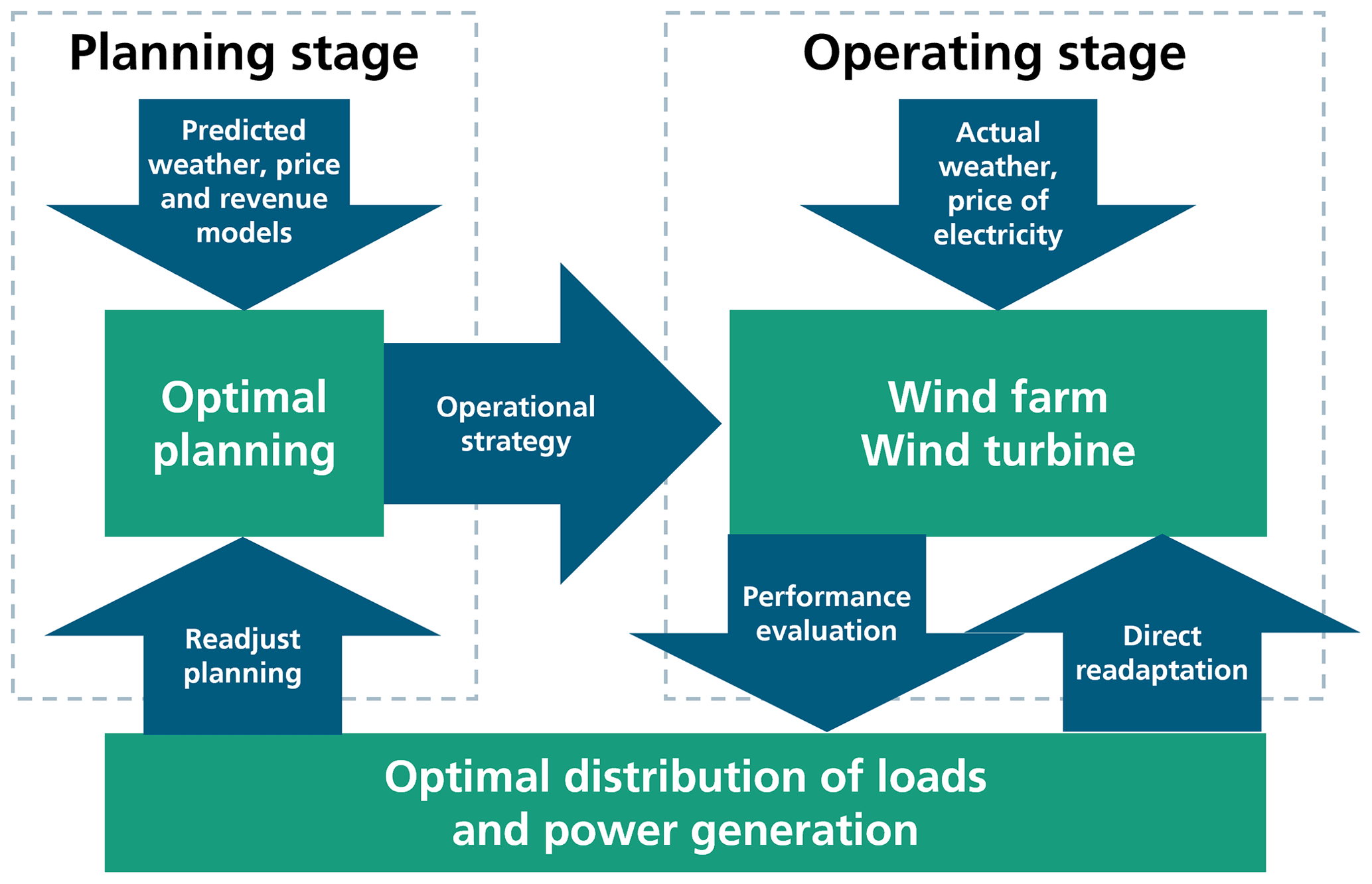
Figure 1Overview of adaptive wind farm operation separated into planning and operating stages.
The long-term objectives for wind turbine operation are specifically driven by fatigue damage progression, which is an important failure mode for wind turbine principal components like the tower and the blades. For an optimal material usage, fatigue budget is ideally fully used up at the desired lifetime while a maximum amount of energy has been produced during this time. Thus, balancing the trade-off between induced damage and power production over the whole range of external conditions and under consideration of their frequency of occurrence is required. The goal is to find a planning method which distributes the fatigue damage optimally over the planned operating time by saving the fatigue budget where it pays off most, i.e. where loads are high but energy production is low. This is possible because of the nonlinear relationship between external conditions, load reducing control features and induced damage. When a turbine is subjected to high wake-induced turbulence, for example, the relationship between induced damage and produced energy is definitely worse than for a turbine operating at the same wind speed at a low turbulence. The key question for an optimally planned target distribution is to decide by how much the damage should be reduced through adaptive control so that the long-term objectives are met. To answer this question, a method to find an optimal planning through mathematical optimization for an individual wind turbine is developed.
1.3 Methodology
In order to create a planning method which fulfils the objectives, the complete process from an adaptation of real-time wind turbine control to the evaluation of long-term goals and requirements needs to be covered. During this process, the influence on damage progression of relevant deterministic external conditions is just as important as that of real-time controller setpoints.
The key part of our proposed method consists of the formulation of a mathematical optimization problem, where the aim is to meet long-term objectives, such as maximum power or revenue over the entire lifetime, by finding an individual trade-off between induced damage and power production for each relevant operational condition.
For application of our method to a given system, it is crucial to know how it interacts with its environment. For this, the system boundary must be well defined beforehand. It forms the basis for definition of environmental inputs, for setpoints of the real-time controller, as well as for the damage of different failure modes and performance measures such as energy production.
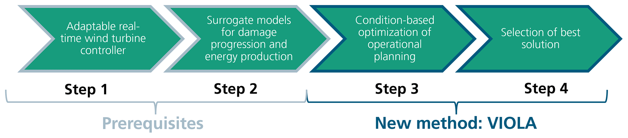
Figure 2Four-step process for optimal planning, subdivided into prerequisites and new method.
We identified a four-step process to create the optimal planning for this well-defined system within its boundaries (Fig. 2). For optimizing the distribution of the fatigue budget over the system's lifetime, it must be possible to evaluate the effect of changes in the setpoints of the adaptable real-time controllers with low computational effort. The setpoints of the real-time controller of the system directly influence the trade-off between induced damage and energy production. Once the adaptable real-time controller is provided, surrogate models can be set up. They represent the relationship between external conditions and setpoints of the controller to damage and energy. These steps 1 and 2 are necessary but existing prerequisites for the long-term optimization of the operation. They need a careful selection and have a strong influence on the quality and the validity of the results. The optimal operational planning is found by steps 3 and 4 of the process. Both of the steps are part of the proposed long-term planning method which we name value-integrated optimization of lifetime asset operation (VIOLA). The optimization problem is developed in step 3. This step still yields multiple results, where each one represents an individual trade-off between energy production and damage. The selection of a single optimal planning becomes possible by evaluating economic aspects of the results from step 3. The four steps not only allow for a feasible computation time, but they also lead to an easily explainable result after each step, which is in high contrast to more integrated approaches. The four steps can principally be applied to any system which is subject to a strong coupling of control setpoints and external conditions. Due to the high influence of wind conditions on the fatigue damage to wind turbines, wind energy systems represent a prime example for its application.
1.4 Outline of the remaining paper
The above-mentioned four-step process forms the core of the remaining paper. At first, the theoretical background and a more in-depth explanation for the approach are given in Sect. 2. The process is demonstrated with an application example. The focus of the example is to effectively reduce power of a considered turbine under conditions where high loads are induced from wake-induced turbulence of neighbouring turbines. In Sect. 3, the considered system is defined. Also, its prerequisites are introduced and implemented, resulting in surrogate models usable for the optimization. Afterwards, the long-term optimization process VIOLA is presented and applied to the example in Sect. 4. The process and the results are discussed in Sect. 5 before the findings are concluded, and an outlook is given in Sect. 6.
The basic idea of our method is to optimally distribute the induced damage over the operating time. With this, we assume a continuous and deterministic increase in damage over time, as depicted in Fig. 3.
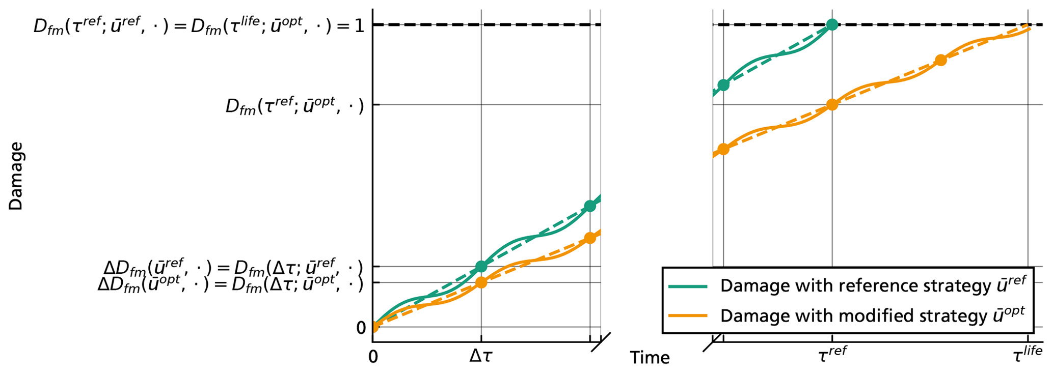
Figure 3Illustration of damage progression over time for a reference (green) and an optimized operational strategy (yellow). Solid lines: representation of continuous damage progression at a time scope of minutes. Dashed lines: linear approximation of damage progression at a time scope of Δτ≈1 year.
Damage always refers to damage which directly and exclusively contributes to a certain failure mode, fm. The lifetime of a system or a component is reached when the damage for a failure mode Dfm reaches the value 1, which is equivalent to 100 % of the available damage budget. Using a reference operational strategy , the value )2 is reached at the reference lifetime τref. Our goal is to use a modified operational strategy over a freely chosen operation period τlife to distribute the damage ) in such a way that maximum energy yield or largest economic profit is obtained. Figure 3 also depicts a time span Δτ, which for wind energy problems is commonly selected as 1 calendar year because it captures the seasonal variations of the wind. Thus, the damage over this time span is referred to as annual damage ) for any operating strategy . Within the time span Δτ, the damage increment on the minutes scope is not constant. Instead, it changes over time due to the variation in environmental conditions and correspondingly varying control setpoints. The continuous damage progression at the more detailed minutes scope is indicated in Fig. 3 by the wave-like behaviour of the increasing damage value (solid curves). This relationship from environmental input conditions and setpoints to damage increment is highly nonlinear in both dimensions, which makes it possible to compensate for high-damage environmental conditions by using low-damage setpoints. For now, the effect of seasonal variation on damage and energy yield is fully included in the final value after the time span Δτ. We use this as the basis of our optimization.
It is immediately apparent that there is a linear relationship between the total damage ) and time τ for any operational strategy . But this holds for given values at discrete time points Δτ only, i.e. for . The value Y is the number of time spans to the full time period τ, i.e. the number of operating years when Δτ represents 1 year with the annual damage being the slope of the linear function. This is expressed by
We now assume that by using an optimal operating strategy , we achieve an optimized lifetime τlife. During this changed lifetime, the entire damage budget is spent, i.e. . The modified lifetime period using is then simply given by inserting the optimized values in Eq. (1) and resolving for τlife:
Thus, our aim is now to find a strategy which optimally changes the annual damage to ).
Computing the modified lifetime with Eq. (2) can result in any time span τlife. However, due to seasonality and the associated nonlinearity within the time span Δτ, Eq. (1) only holds true for Y∈ℕ. This applies for τref, but the resulting value τlife from Eq. (2) depends on the optimized damage increment ) and can take up any value. It is in turn not restricted to natural numbers. For a long time span τlife, the resulting error is small in comparison with uncertainties resulting from the assumptions for the deterministic long-term fatigue modelling approach.
That the assumption
holds is due to a suitable scaling of ). Among other things, this includes the assumptions that the damage budget is completely used up under the reference strategy and that the damage increment is always the same for each time increment Δτ. The latter is based on the standard approach in the design process of wind turbines, where the damage increment of a short time interval Δt (10 min to 1 h) is extrapolated to the annual damage progression using a frequency distribution of the input conditions, i.e. to the time periods Δτ and τlife respectively. Therefore, the damage increment dfm(x,u) under the external input conditions x∈X and the control setpoints u∈U needs to be known. Here, X defines the space of selected input conditions for the specified system boundaries and U is the space of possible control setpoints. In principle, dfm(x,u) can be obtained from an arbitrary method for a specific failure mode. In this work, we use the standard approach for wind turbine fatigue modelling based on the assumption of a linear damage accumulation by Palmgren and Miner (1945, Sutherland, 1999).
For the long-term calculation of damage and fatigue, different time scopes are relevant. Figure 4 shows an overview of the different time scopes in interaction with the surrogate models. It also gives an overview of terms and symbols used. For the surrogate models, inputs and outputs on the minute scope are decisive. The relationship between in- and outputs is created by using high-fidelity simulations on the seconds scope and evaluating their time series into a single value. At the seconds scope, the control setpoints u are transferred into the real-time controller of the wind turbine. Multiple simulations of this type are carried out to create the surrogate models. Thus, the creation of the models finalizes the required prerequisites of steps 1 and 2 according to Fig. 2. The optimization process is later carried out on the annual scope, where the surrogates are evaluated to calculate the annual damage and the annual energy depending on different operational strategies. Finally, the annual values can be used, to compute the lifetime total energy and total damage. Before those can be used for the long-term optimization process in steps 3 and 4, we explain the relationship between the different time scopes with respect to loads, fatigue damage, lifetime and energy production on a theoretical level.
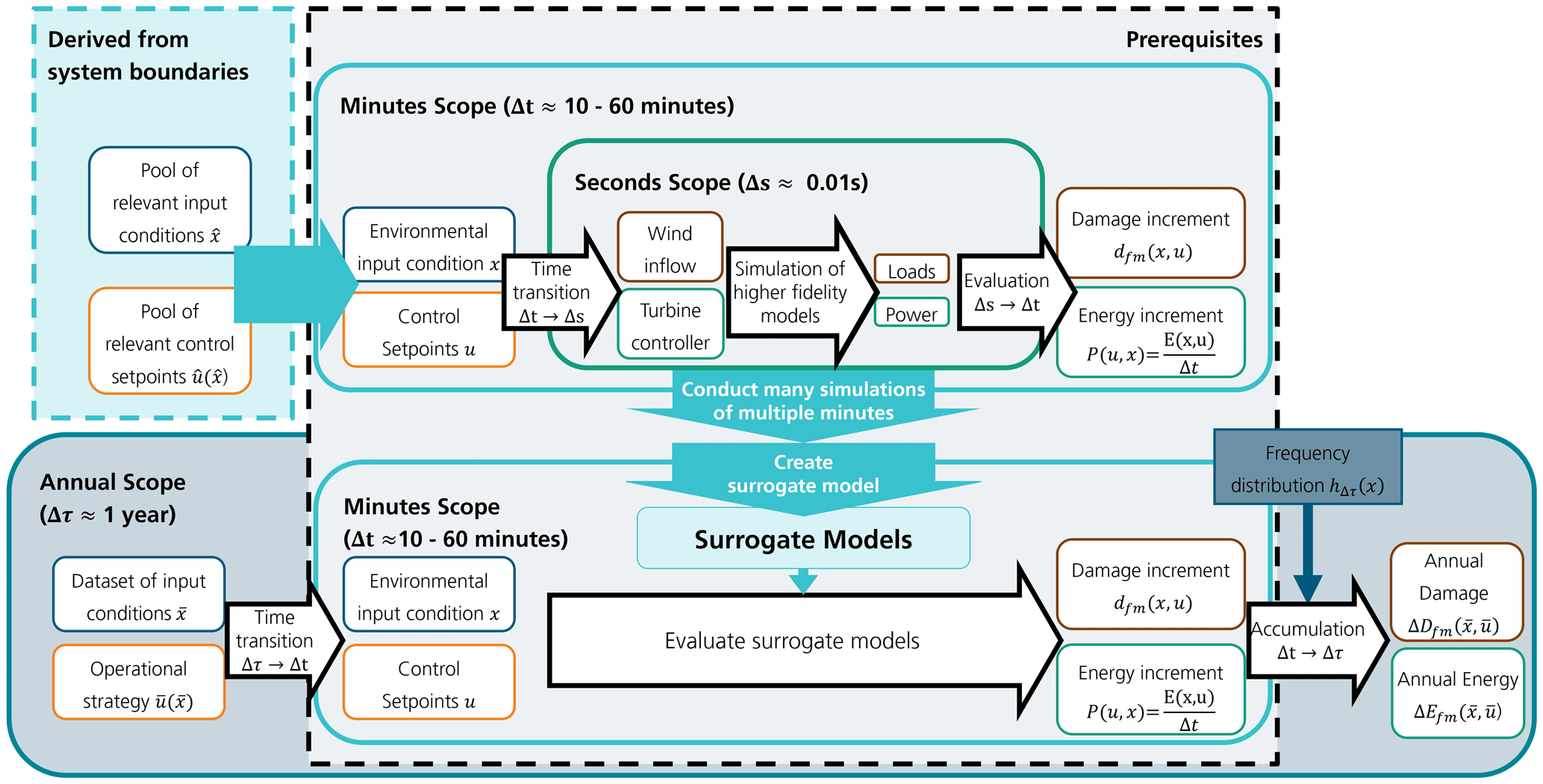
Figure 4Overview of time scopes for creation and usage of surrogate models. The white rectangles with rounded curves denote in- and outputs on different time scopes. The white arrows describe a transition from input to output with a corresponding model. The rectangle in the centre contains the prerequisites and ends with the creation of surrogate models which can be evaluated on the minutes scope. The creation process is depicted by the cyan arrows, starting from the pool of input samples. Within the annual scope, the surrogate models are used to compute the annual value with the frequency distribution as an additional input.
2.1 Long-term fatigue damage progression and energy production depending on external conditions and operational planning
The standard approach in wind turbine design is the extrapolation of wind turbine loads from simulations to the design lifetime of, for example, 20 or 25 years. It is also a requirement for the certification of a turbine, defined in standards like (IEC, 2019; DNVGL-ST-0263, 2016). In the standards, design load cases (DLCs) determine the external conditions. To cover a wide range of sites, reference classes of wind conditions are defined, and conservative assumptions are often made. Currently, a fixed operational strategy is assumed for each turbine. The major difference between standard design calculations for fatigue damage and the presented approach for optimal planning is the explicit integration of the control setpoints as a dependent variable on the external conditions, which can adaptively be selected and thus used as an optimization variable. To cover the dependency of control on the external conditions, we assume that for each external input condition x∈X, there is one setpoint or multiple setpoints for the real-time controller u(x)∈U that can be selected. Both, input conditions and control setpoints, are defined on the minutes scope and thus valid over the time increment Δt, i.e. between minutes and hours. To determine the relative frequency for each combination of input conditions, binning is required. Each combination of conditions is allocated to a separate bin j. The vector of input conditions is denoted as xj for a corresponding bin , where Bx is the total number of all bins of all input conditions.
The dimension of xj is given by the number of input conditions w=Dim(X). The entire set of input conditions is denoted as . For each combination of input conditions, a separate operational strategy, i.e. setpoints of the system within the specified system boundaries, , is defined. The total number of bins Bx is usually defined as a full-factorial multiplication , where denotes the number of bins defined for each condition x(i).
In order to extrapolate the effects of the input conditions over long periods of time, a relative frequency distribution pΔτ, which is representative of the input conditions within a period Δτ, is usually used. Hence,
which can be scaled to an (absolute) frequency distribution,
for a time period
For wind turbines, an annual distribution for the wind conditions, i.e. Δτ=1 year, is able to represent the variations through the different seasons. With the frequency distribution and the planned operational strategy, a damage ) can then be determined over the period Δτ, i.e. an annual damage progression assuming an annual wind distribution.
Using this and the assumption of a linear damage accumulation, damage can also be defined as a function of τ depending on the defined frequency distribution over that period and the operational strategy,
where dfm(x,u) is the damage increment under the external input conditions x and the control setpoints u. It is also possible to compute the energy production accordingly by
where is the energy increment under the input conditions and ) the average annual energy within Δτ.
With adapted operational control for modified lifetime, the time period over which energy is produced is changed as well. The total lifetime energy yield can be computed by introducing a lifetime extension factor. It relates the lifetime with the reference operational strategy to the modified lifetime:
Until now, the resulting lifetime was denoted as τlife, but in fact, this value is computed from damage Dfm(⋅) relevant for a certain failure mode, fm, and thus also only valid for this specific failure mode. For this reason, hereafter it is denoted as ) and the extension factor as ). With this, Eq. (9) can be expressed as
The deterministic lifetime extension factor ) can thus be used to compute the potential for lifetime extension on any time period where the damage increment is compared for two different strategies.
Then, the energy production from the optimized operational strategy is given by
Within the course of this work, ) is later used within the optimization process. It is important to realize that this value is actually closely related to the damage computed with the reference strategy. This becomes more clear when the damage increments are connected to the fatigue damage budget. Up to now, the assumed damage progression is applicable to any failure mode where damage accumulates over time. With this, we implicitly also assume that the details about material properties of the specific failure mode are included in dfm(xj,uj).
2.2 Relationship between fatigue damage and damage equivalent load (DEL)
Fatigue damage is typically based on the linear damage accumulation by Palmgren and Miner (1945). Especially for the comparison of loads under different environmental conditions or control approaches, it remains a useful approach as a first step before more advanced evaluations can be examined with further development. For the explanation of the general process, the failure mode index, fm, is dropped. The fatigue damage increment of a load time series simulated on the seconds scope, with input conditions xj, is given by
for i effective load collectives with a number of load cycles ni. Ni denotes the maximum bearable number of load cycles until failure for the corresponding specific oscillation amplitude. The number of load cycles counted in the load time series of length Δt is denoted by ncyc,j. The tolerable number of load cycles Nij depend on Dult and can be determined with
Lij represents the oscillation amplitude of a load cycle and are usually obtained from a rainflow counting algorithm. The parameter m is the component specific Wöhler exponent describing the slope of the S–N curve as negative inverse on a double logarithmic axis. In the formulation of Eq. (13), the mean load is neglected and no Goodman correction is performed. The value Dult denotes the ultimate design load which would lead to a damage of D=1 if it occurred once. Therefore, Dult is a design parameter which needs to be determined from the design process under consideration of all conditions and their frequency for the desired reference design period τref. In addition, it normally includes safety margins and design reserves. For simplification Dult can be scaled in such a way that
is valid, i.e. that fatigue damage is fully utilized with the reference operational strategy and under some site-specific reference frequency distribution:
In this case, Dult can be expressed by making use of the damage equivalent fatigue load (DEL). It is a representative value which would yield the same damage as the considered time-varying signal with a constant amplitude and frequency. This value is related to an equivalent number of load cycles Neq. Then, the short-term DEL is computed by
and the total DEL over the time span τ is given by
This can be used to solve Eq. (14) for Dult:
This can subsequently be inserted into Eq. (13) so that the damage can be expressed using the DELs as a relative value:
In order to model the nonlinear damage increment for the external conditions, surrogate models can be created by using the relationship to the short-term DELs which is given by Eq. (19). In principle, surrogate models for the damage increments could directly be computed, but creating the models for the DEL is more common and easier to interpret because the Wöhler exponent m adds additional nonlinearity to the damage value.
Based on the theoretical background for fatigue calculation, the four-step process will be applied to a specific use case. Therefore, the system boundaries for the exemplary use case will be defined first. Afterwards, the first two steps of the process are explained and applied to the example.
3.1 System boundaries for application example
We focus on optimal operation of a single turbine within a wind farm. This means that effects from the surrounding wind farm have to be taken into account as well. These include mainly the wake effects from other turbines, which act on the considered turbine and are, under normal operation, a significant driver of its loads. Each single considered turbine will thus be able to react to the wake effects from the surrounding turbines, but the effect from changes in control on the wake cannot be considered yet.
3.1.1 Modelling of a single turbine and its system boundaries
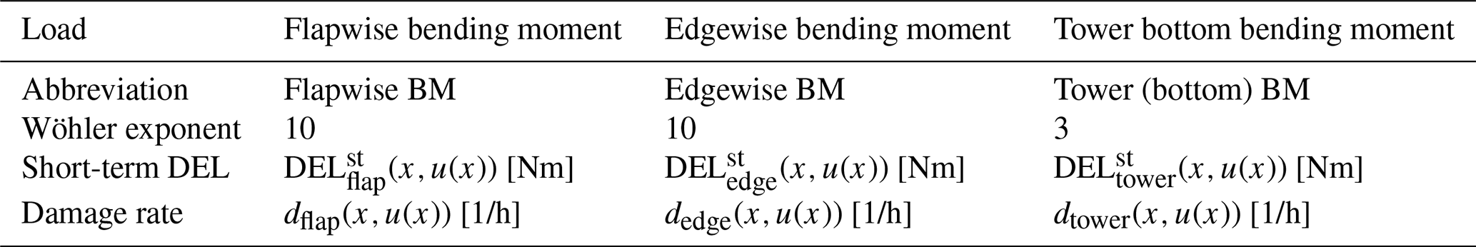
The generic direct-drive wind turbine IWT7.5 with a nominal power of 7.5 MW, rotor diameter of 164 m and a hub height of 100 m is used (Popko et al., 2018). To compute the loads of the turbine on the so-called seconds scope (Δt= 0.01 s), the aero-elastic load simulation tool “The Modelica Library for Wind Turbines” (MoWiT) (Thomas, 2022) is employed. Three-dimensional wind fields covering the properties of the external conditions for each simulation are used as input. They are created with the software Turbsim (Jonkman, 2009). MoWiT is developed at Fraunhofer IWES as an object-oriented library for fully coupled aero-hydro-servo-elastic simulations of wind turbines. Detailed information on the development of MoWiT can be found in the literature (Thomas et al., 2014; Leimeister and Thomas, 2017). The tool covers on- and offshore turbines with bottom-fixed substructures, and also floating wind turbines. It is coupled to the adaptable controller outlined in Sect. 3.2. Two major environmental inputs influencing the wind turbine loads in power production mode are considered as local input conditions: mean wind speed v and turbulence intensity at hub height turbulence intensity (TI). Those input conditions are defined locally as the inflow to a single turbine which positioned its rotor perpendicular to the main inflow wind direction. All other parameters which define the inflow wind field, such as vertical and horizontal wind shear, are fixed at their IEC-standard values. The local inflow on a turbine from wake effects is covered through an increase in turbulence intensity only and does not include wake meandering effects. This simplification allows splitting the aero-elastic turbine simulations from the wake modelling, and thus reduces simulation effort. Considering other effects like wake meandering for the creation of surrogate models is possible through an extension of the load simulations but goes beyond the scope of this work, because the major effect of an increase in loads is covered through the applied approach. For the demonstration of the approach, the structural loads of the blades and the tower are considered. Both are supposed to last for the complete design lifetime of 20 or 25 years. Both are also influenced by the turbine controller and the wake-induced turbulence. For the blades, the flapwise and edgewise bending moments (BMs) are considered as separate failure modes, because they represent the two major load driving moments on the rotor blades. For the tower, the combined bending moment at the bottom is utilized as failure mode. All these loads can be considered as representatives for the fatigue accumulation of different components that can be influenced by the wind turbine controller and the environmental conditions in different ways. While the tower and the flapwise bending moment are more strongly influenced by turbulence, the variations in the edgewise BM are driven by gravity loads dependent on the rotor speed, i.e. the controller and the wind speed.
The considered loads, their corresponding abbreviations and the utilized Wöhler exponent m are summarized in Table 1. Using linear fatigue accumulation by using DEL is a very strong simplification for the fatigue degradation of laminate, which is a composite material containing fibreglass. Using this approach is still standard for design calculation and allows for straightforward use without detailed knowledge about the material properties. For the tower, an exponent of m=3 is used, which is representative for steel components and m=10 for the blade loads as an approximate for fibreglass (Sutherland, 1999).
3.1.2 Wind farm setup: from surrounding system to considered wind turbine
The influences of the surrounding system on the considered wind turbine are covered by a site-specific wind distribution and the wake influences from the surrounding turbines in the wind farm. The wind farm consists of nine turbines with a regular 3×3 layout, shown in Fig. 5a. It was already used in Schmidt et al. (2021). In this work, we optimize operational strategies for the turbine in the centre (index 4). In doing so, we can put a focus on the method for operational planning and the discussion of derived results. There are various studies and models to illustrate the effects of wakes on the loads, ranging from wake meandering to partial wake effects (Mendez Reyes et al., 2019; Nash et al., 2021). Since the core of this work lies in the optimization methods, we limit ourselves here to a simple steady-state modelling of the wake effects for wind and turbulence, which cannot cover these effects yet. For this purpose, we use the IWES software FOXES (Schmidt, 2022). The local wind speed is computed using the Gauss-type wake model by Bastankhah and Porté-Agel (2016). The wake-induced TI is calculated using the top-hat wake model as described in IEC (2019). For the ambient TI, we use the wind-dependent Weibull distribution according to IEC (2019) with class B at the 50 % quantile to cover the mean effects at such a site. For the superposition of wakes, we use a linear superposition for the wind speed and the maximum superposition for TI. Local TI depending on the ambient wind speed and direction is shown in Fig. 5b.
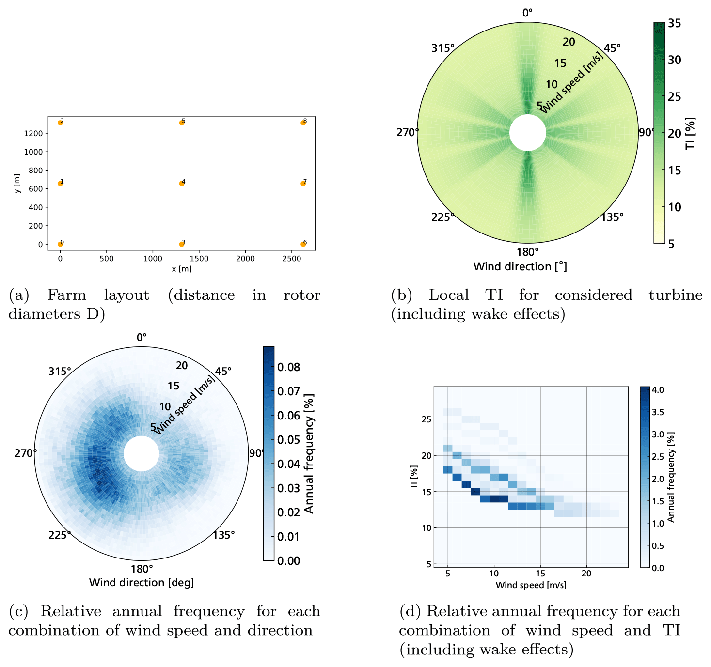
The annual frequency distribution is derived from a 30-year time series of ERA5 data in the North Sea with a resolution of 1h from 1990 to 2019 (Hersbach et al., 2018). The mean wind speed and wind direction at 100 m height are extracted to create a relative frequency distribution of ambient wind speed and wind direction , which are both subdivided into bins. Therefore, the reference relative wind distribution for the ambient wind conditions is ) with Δτ=1 year. Because wind speed and direction are covered separately, the total number of bins Bx is subdivided into bins for each direction. The wind speeds are first binned with a resolution of 1 m s−1 from 1.5 to 49.5 m s−1. Only values within the operating envelope of the turbine (4.5 m s−1 m s−1, number of wind speed bins ), where derating can influence the turbine, are considered for optimization. It also means that ) does not sum up to 1 anymore. The wind direction is binned with a resolution of 2∘ from 0 to 358∘ (Number of wind speed bins ). This results in a total number of bins. The percentage annual frequency for those bins is shown in Fig. 5c.
For a single turbine, the wake model represents a function which maps the ambient mean wind speed vamb and wind direction θamb to the local mean wind speed v and turbulence intensity TI. Since the interaction of the turbines is only modelled unidirectionally, without considering the influence of the changed control setpoint on wake towards other turbines, it is possible to create a local frequency distribution for each turbine, which only depends on the distribution of local wind speeds and turbulence. To do so, the frequencies of ) are binned again into Bv=20 wind bins, as before, and BTI=25 TI bins with a width of 1 % starting from 5 %, resulting in 500 total bins. The frequency distribution for the additional binning is denoted as and is only valid separately for each turbine in an arbitrary wind farm with S turbines. The local frequency distribution of the centre turbine 4 is shown in Fig. 5d. The TI values increase from the ambient TI, which still shows the highest relative frequency. The frequency of TI values increases for certain combinations, as indicated in Fig. 5b. Then, the damage and energy calculation can be derived:
and
This simplified form, which adds uncertainty to the optimization result, will be used in the results part during application of our approach. The uncertainty can be influenced by the number of bins selected. It can be well estimated in comparison with the original binning and lies below 1 % for the considered cases.
3.2 Adaptable real-time controller of the wind turbine (step 1)
The primary objective of a wind turbine controller is to maximize power production while meeting the requirements of a grid operator (Burton et al., 2011; Njiri and Söffker, 2016; Requate et al., 2020). Additionally, secondary objectives, such as load reduction, are pursued during control design. This can be achieved, for example, by implementing features for reduction in loads on specific components. Examples are exclusion zones to reduce tower vibrations or individual pitch control (IPC) to reduce fluctuations in blade root bending moments. However, these secondary objectives usually force the controller to deviate from optimal operation with regard to its primary objectives. Some secondary objectives might even compete with one another, e.g. blade root loads and pitch actuator activity for IPC. We now assume that the balance between primary objective and secondary objectives can be selected externally by adapting the controller through a control setpoint.
In Sect. 2.1, we already introduced the control setpoint as u(x). We assume this to be an abstract value which can be selected based on the external input conditions x. Thus, u is a vector of controller setpoints, which in turn reacts by adjusting its own internal parameters. In a larger wind farm system, which is composed of multiple turbines, which uses wake steering or wake reduction, u(x) could be the yaw angle or the amount of power derating (Nash et al., 2021). Within the remainder of this paper, we assume a one-dimensional control setpoint for the power derating of a single turbine. This is a commonly available input, as reduced power capability is also requested by grid operators to mitigate grid congestion. There are several studies which investigate derating methods with respect to various objectives. These methods include power regulation for the grid, wake reduction or loads. In Houck (2022), several studies on derating (or axial-induction control) are summarized and sorted into the mentioned categories. Many studies investigate load reduction as a side effect, while the main objective is either the power regulation or reducing the wake on the downstream turbine.
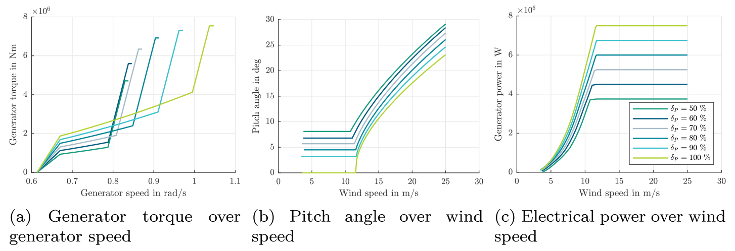
Within the system boundaries of this study, the main objective is not to determine the best fitting derating method for the generic wind turbine, but to show the benefits of using derating for an optimal planning. Therefore, the choice is conducted based on the findings from the literature and from previous experience with the generic IWT7.5 wind turbine, and not through an extensive study and tuning of the controller under various conditions. Also, no additional features, such as individual pitch control or active dampers, are activated. For a real-world application, fine-tuning the controller for every derating configuration would be beneficial and could lead to an improved performance with respect to loads and power. The IWT7.5 is controlled with the IWES research controller (Wiens, 2021). The derating method is implemented such that it reduces power in partial and in full load by a percentage factor δP∈ []. Such a derating method is referred to as proportional delta control in Elorza et al. (2019) or percentage reserve in van der Hoek et al. (2018).
In partial load, both tower and blade fatigue loads should be decreased. To do so, the constant-λ method is implemented (Astrain Juangarcia et al., 2018), because we expect a positive effect on these loads based on the literature, and we avoid potential negative effects like a near-stall operation as, for example, by using the minimum-thrust strategy. This is achieved by finding the steady-state pitch angle β so that the reduced power coefficient δPcp is found while λ is kept constant. From these values, the parameters for derated operation can be computed.
In the full load region, the torque setpoint is normally reduced for derating. This allows for a fast recovery of power when derating is no longer required, and is thus beneficial for ancillary services (Fleming et al., 2016; van der Hoek et al., 2018). However, it only has a minor effect on the fatigue loads of the blade and the tower. Reducing the generator speed mainly has a strong positive effect on the blade loads in the flapwise direction (Requate and Meyer, 2020), while reducing the torque has a positive influence on the driving torque loads (Pettas et al., 2018). The effect on the tower loads are quite turbine dependent because a reduction in generator speed can reduce oscillations to some extent but often also increases them due to the lowered aerodynamic damping (van der Hoek et al., 2018). Therefore, a mixed method between reducing torque and speed might be advantageous, again depending on individual objectives and turbine characteristics. Both methods are combined for reducing the rated generator torque Mr and ωr.
In Fig. 6, the operating points of the controller for the selected setpoints are presented. Figure 6a shows the speed–torque curve of the controller. The end point of the curves always determines the combination of Mr and ωr. By comparing the progression of these curves, the effect of both strategies can be observed. In partial load, the constant-λ strategy determines a specific combination of parameters including the static pitch angle. The steady-state operating points of the pitch-angle are plotted over the wind speed in Fig. 6b. In combination, this results in the steady-state power curves which are shown in Fig. 6c.
The control setpoints can then be used as optimization variables in the formulation of a mathematical optimization problem. However, using them directly within an optimization requires full simulation of respective load cases, which is not feasible due to the required computational effort. Instead, surrogate models can be set up which abstract the whole turbine–controller interaction.
3.3 Surrogate models for damage progression and energy production (step 2)
Surrogate models, sometimes also called meta-models, are a necessary prerequisite for evaluating and optimizing different influences on damage over long periods of time. For wind turbines, they have gained growing research interest to cover the influences of various external conditions and control on fatigue damage. They have in common that aero-elastic simulations are used to create a database of fatigue loads for various input conditions. In Fig. 4, those aero-elastic simulation models are denoted more generally as higher fidelity models on the seconds scope. The surrogate model is created by performing multiple simulations for a pool of input samples. Due to the relationship between damage increments and DELs, the surrogate models can be calculated on the basis of the short-term DELs. Thus, the strong nonlinearity due to the Wöhler exponent does not have to be considered, and the damage increments can be calculated using Eq. (19). The short term DEL ) is obtained through aero-elastic simulations of the wind turbine model and a subsequent evaluation using the rainflow counting algorithm and Eq. (16).
By using surrogate models to compute damage and energy increment, additional uncertainties are inevitable when calculating long periods of time. At the same time, the load calculation of wind turbines is always associated with uncertainties due to the stochastic influences of the wind (Mozafari et al., 2023). This must be taken into account when creating surrogate models. Depending on the application and effort, different requirements are made on the surrogate models. For example, more accurate models are required for fatigue tracking or for calculating the remaining service life than for use in an optimization. Here, fast evaluation and good mapping of the correlations between optimization variables and initial values are of particular importance.
In this work, the surrogate is considered as an existing prerequisite with various suitable approaches from the literature ranging from Gaussian regression (often referred to as kriging) to polynomial chaos expansion to artificial neural networks (Dimitrov, 2019; Hübler, 2019; Slot et al., 2020; Gasparis et al., 2020; Debusscher et al., 2022; Singh et al., 2022). A good overview of different surrogate methods and a comparison of their performance is given in Dimitrov et al. (2018). Despite their known lower accuracy compared with some of the other methods, we select multidimensional polynomial regression models for the DELs due to their suitability for optimization, their simple usage, their differentiability and their fast training and evaluation time. For the electrical power, a linear interpolation is used.
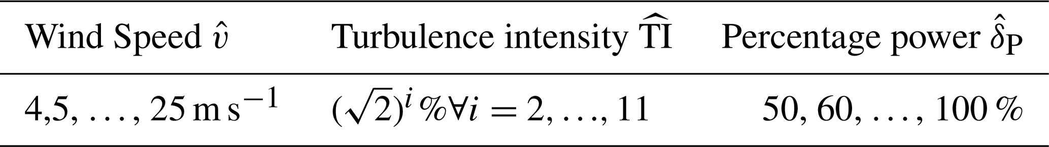
The pool of input conditions is created with a full-factorial sampling for the wind conditions x together with the percentage power u(x)=δP(x). The sampling values are provided in Table 2. While wind speed and power are sampled equidistantly, the sampling of the TI values is selected so that the distance between the samples increases exponentially, as indicated by the formula in Table 2. This reduces simulation time and still creates enough data in situations with high occurrence. To account for the randomness in the incoming wind, various realizations of the same mean input characteristics are usually simulated; those are determined through pseudo-random seeds. For the simulations performed in this work, 6 simulations of 10 min on the seconds scope are performed to obtain a damage increment on the minutes scope with the time increment Δt=60 min = 1 h as is standard for DEL calculations.
To obtain the parameters of the polynomial regression model for the DELs, a least squares approach is used. The maximum order of the polynomial is set to 5. The value is found by cross validating different orders of the polynomial between 1 and 8. For the further usage of the surrogate models, it is particularly important that the influence of the derating setpoint at the different input condition be correctly represented. For all three failure modes, a general agreement of the surrogate model to the data can be observed. Figures 7 and 8 exemplarily show the evaluated surrogate model (solid lines) as well as the simulated training data (dots in same colour as solid line) when one of the input conditions is set to a fixed value. The DELs are normalized with respect to the fixed values (v= 8 m s−1 and TI =16 %) at the nominal percentage power δP=100 %. The power is not explicitly shown here because its behaviour, dependent on wind speed, directly derives from the control setpoints (cf. Fig 6c). In general, the accuracy of the fit for the flapwise BM and the tower base BM is lower than that of the edgewise BM. These loads are more strongly influenced by the turbulence of the wind and thus also have a higher uncertainty in the simulated DELs. Especially for the tower, the high variation in the simulation data makes it difficult to create a surrogate model. Also, the relative mean error on the complete dataset is highest for the tower BM (error = 3.88 %), compared with the error in the flapwise BM (2.32 %) and the edgewise BM (0.23 %).
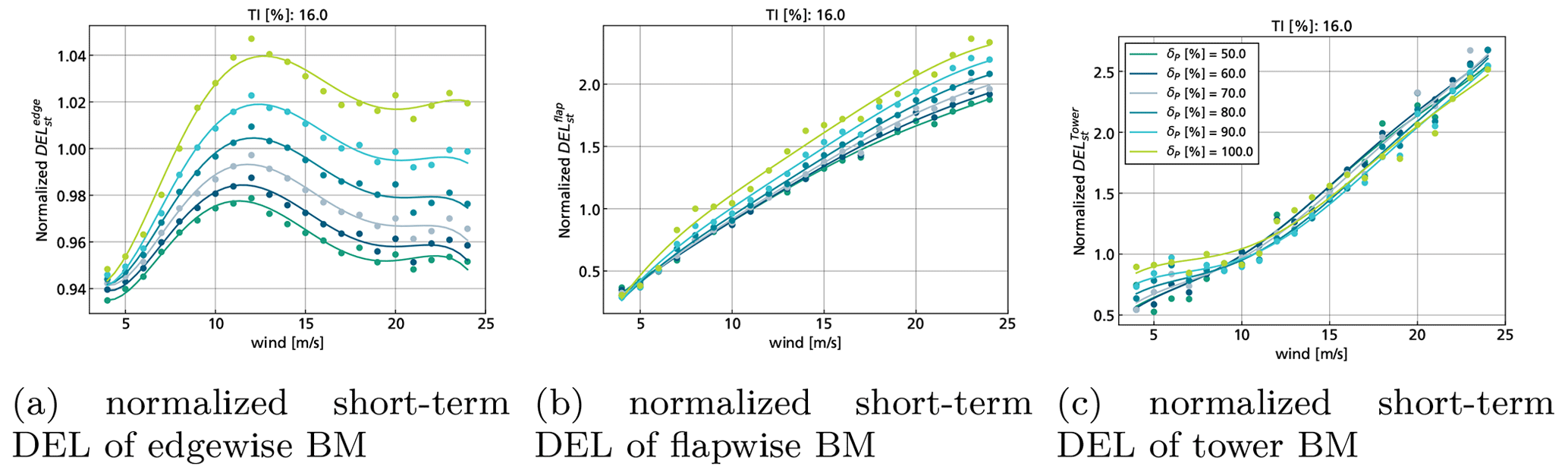
Figure 7Evaluated surrogate models (solid curves) and simulated data points (dots) for a fixed TI of 16 % normalized with the short-term DEL of the nominal strategy δP=100 % at v = 8 m s−1 and TI = 16 %.
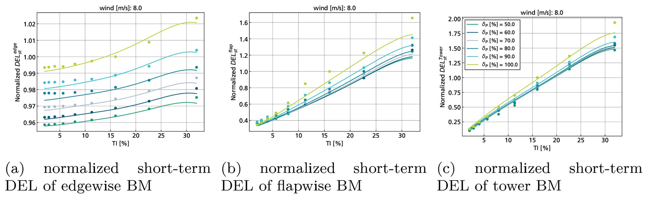
Figure 8Evaluated surrogate models (solid curves) and simulated data points (dots) for a fixed wind speed of 8 m s−1 normalized with the short-term DEL of the nominal strategy δP=100 % at v = 8 m s−1 and TI = 16 %.
The behaviour of the DELs depending on the control setpoints will now be briefly discussed. Figure 7 shows the results with the wind speed v on the x axis for different values of percentage power δP=100 % with a fix TI = 16 %. Both, the flapwise and the tower DELs ( and ), strongly increase with the wind speed (cf. Fig. 7b and c), while the DELs of the edgewise BM reduce when the rated wind speed is reached at 12 m s−1 and the turbine starts pitching (cf. Fig. 7b). The reduction in depending on δP=100 % directly relates to the lower rotational speed through the control setpoints at each wind speed. Thus, it has a stronger effect at 90 % and 80 % when the rotor speed is lowered by a higher amount than the generator torque to achieve the power setpoint. The decrease in is also rather small compared with the other two failure modes, where the relative difference in DELs is much higher. The can be reduced for almost all wind speeds (cf. Fig. 7b), but not by the same amount. The DELs of the tower BM show a much less clear relation to the percentage of power. For low wind speeds, the values of also decrease with the lower values of δP=100 %, but with some significant variation within the simulated data points. For higher wind speeds, reducing the power can even increase the tower loads, and the relation is not completely deterministic. This effect is caused by the reduced aero-dynamic damping due to the rotor speed reduction or from resonance effects.
Figure 8 shows results with TI on the x axis for different values of δP with a fix wind speed v= 8 %. The is not significantly influenced by the turbulence. The load reduction in the edgewise DEL is low compared with the other two failure modes. For the flapwise bending moment and the tower bending moment, the strongest relative reduction can be achieved by reducing the power to 90 %, but more derating still decreases the DELs slightly further. The relative load reduction also increases with increasing turbulence.
The results presented in this section show several aspects which are relevant for the optimal planning approach. The selected method for derating is suitable to reduce the short-term DELs and thus the damage increments of all the failure modes. Also, the surrogate models are able to cover the nonlinearity sufficiently to be used for further optimization. The optimal planning approach can make use of this to determine when a load reduction should be favoured over a higher energy production. This can especially be done by exploiting the fact that higher turbulence significantly increases loads, but the power production remains almost the same. This effect is even strongly enforced from the relation of the short-term DEL to the damage increment because the value is raised to a higher power by the Wöhler exponent (see Eq. 19).
Having created the surrogate models depending on the selected control setpoints as prerequisites, they can now be used to determine how much derating is beneficial to apply, through the optimal operational planning method. The process for the assessment of lifetime objectives dependent on the operational strategy is shown in Fig. 9. The lifetime objectives are modelled by making use of the surrogate approach on the annual scope. The total damage determines the lifetime of the wind turbine, which influences total energy production and total value. While the total energy and damage define the objectives on a technical level, maximizing the total value is the final goal. All objectives are influenced by the setpoints for the operational strategy, which determine the optimization variables. The key of the method is to formulate the problem in such a way that a control setpoint is found for each external condition while these long-term objectives are fulfilled. We refer to value as a general measure for the overall valuation of the considered wind energy system. It will usually contain an economic valuation but may also include other factors such as environmental impact or contributions to grid stability. We call the framework for this method VIOLA (value-integrated optimization of lifetime asset operation). The process shown in Fig. 9 forms the basis for the formulation of the optimization problem which currently consists of the two separate steps, namely steps 3 and 4, of the complete process (cf. Fig. 2).
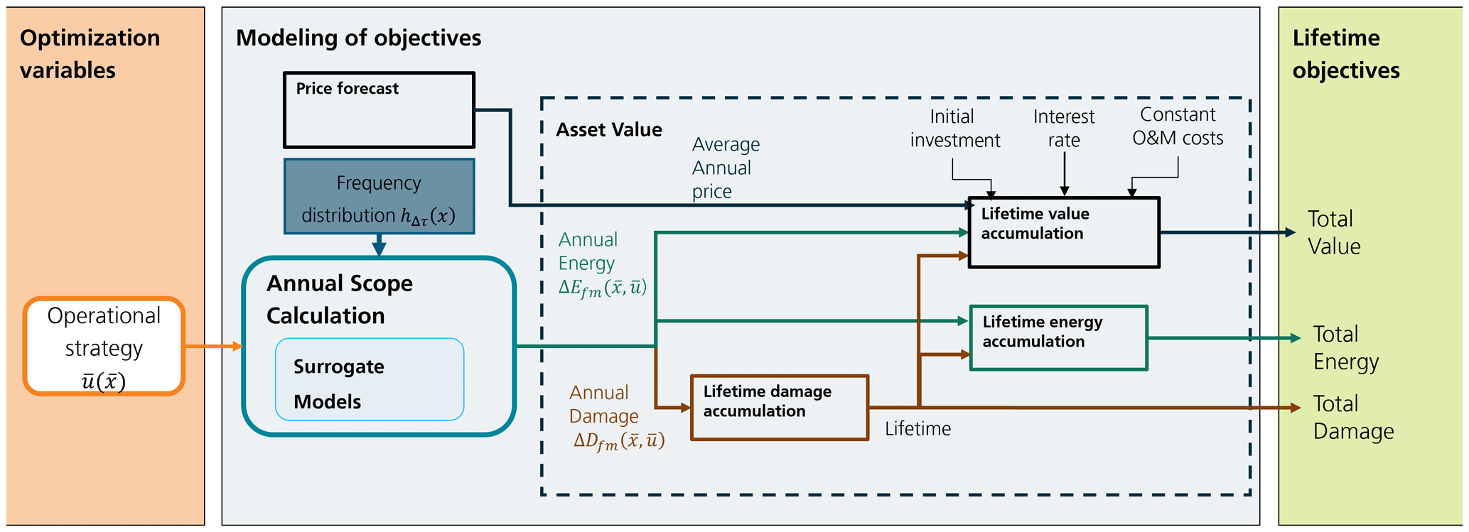
Figure 9Process for computing the lifetime objectives dependent on operational strategy. The setpoints of the operational strategy define the optimization variables. They are input to the annual scope calculation based on surrogate models and frequency distribution. With the output of this calculation, annual damage and annual energy can be accumulated to a lifetime value. The lifetime is determined from the total damage and thus used as an input for lifetime energy and lifetime value accumulation. The lifetime value is computed with additional inputs for the specified value metric.
4.1 Condition-based optimization of operational planning (step 3)
Developing the mathematical optimization process for finding the operational strategies is the central part of this work. Neglecting economic factors and other influences and restrictions for the total value of a farm at first, it is ecologically most beneficial to get the maximum amount of energy over the lifetime τlife of the turbine while the fatigue budget of each component is fully used up. Therefore, the total energy for a given target damage budget is maximized over the fixed reference time τref. The operational strategy is optimized for each of the external conditions which were previously selected by the definition of the system boundaries. It follows that the number of selected independent control setpoints, defined by Dim(U) and the number of bins which are used for the external conditions Bx, determine the number of optimization variables, which is equal to Bx⋅Dim(U). Within the scope of this work Dim(U) is equal to 1 because a single derating strategy will be applied. With a fixed known target fatigue budget for failure mode fm∈ℱ, the optimization problem is formulated as
Using this simple and compact formulation, it is possible to spare the fatigue budget when the damage increment is high compared with the energy increment. When the damage of all failure modes is reduced compared with a baseline operation , i.e. , the turbine can be operated for a longer time and ultimately more energy can be produced.
The optimization problem is solved by using the gradient-based interior point algorithm for constrained nonlinear optimization problems (Waechter and Laird, 2022). The process itself is formulated with Python and the optimizer is interfaced through the library pygmo (Biscani and Izzo, 2020a), which builds on the C++ library pagmo (Biscani and Izzo, 2020b). Gradients are computed using finite differences. Optimization runs were executed on a laptop with an Intel i7 four-core processor, 2.1 GHz speed and 32 GB RAM. The execution time of each run ranges from several minutes to several hours, depending on the specified target damages. The optimizer typically needs between 100 and 500 iterations to converge. As starting values, the reference strategy with 100 % power production at each turbine was always used, which is a nonoptimal but feasible solution. All optimization runs show plausible results in terms of an improved relationship between the energy increment and damage increment. For this reason, no explicit variations of the starting values were required to check for convergence to local minima.
Clearly, the solution strongly depends on the selected failure modes, their behaviour with regard to the damage rate determined from the surrogate models and on the target fatigue budget. When several failure modes should be optimized simultaneously, it might be impossible to fulfil the constraints and no solution can be found. Therefore, the selection of the target budget strongly depends on the specific problem which relates to a specific wind farm or wind turbine. The formulation in Eq. (22) provides a clear separation of the technical aspect from the economic aspect and therefore allows investigating the relationship between damage progression and energy production for different components under consideration of the operational strategies over long periods of time. It can also directly be used to create a Pareto front between damage and energy production by principally applying the epsilon constraint method for multiobjective optimization (Chiandussi et al., 2012), i.e. by fixing various combinations of the target values . We pursue this approach in this work and select a specific strategy based on further information in the final step 4.
4.1.1 Creating Pareto-optimal solutions for the application example
We apply the optimization method to the considered turbine in the centre of the wind farm. To do so, we first need to define the reference design value DELref. It is computed with the site-specific wind distribution, including wake effects for wind and TI, and with the reference operational strategy . This means that operating with the reference strategy yields a damage value of 1 for all failure modes after the nominal operating period. This implies a site-specific design, where all components are designed for the local site conditions. This strong assumption stands in contrast with series manufacturing of turbine components. However, it allows a simpler interpretation of the results at this point. We limit ourselves to the factors that can be influenced beyond design decisions and safety factors. Therefore, each reduction in damage of a failure mode results in an extended lifetime according to the deterministic assumption from Eq. (10).
By solving the problem for various values of , the maximum amount of energy for each of these values can be found. For simplification, each failure mode is considered separately. On the one hand, this increases the interpretability of the results. On the other hand, it would be applicable if the weakest failure mode of a turbine or component can clearly be determined. For each failure mode , at first the minimum possible damage is computed as an orientation. Then the optimization problem
is solved with constraint between 0.3 and 1 depending on the failure mode to obtain desired points the three Pareto fronts. Each point yields an optimal planning strategy separately for each failure mode. Such a strategy is denoted as .
The results of the optimization, i.e. the Pareto fronts, are shown in Fig. 10 where the relative percentage energy production compared with the reference case is plotted over the total damage, which is equal to 1 for the reference case. When comparing the results, one can clearly see the different behaviour of the failure modes, which results from the determined relation of the damage rates to the control setpoints and the external conditions. While it is possible to significantly decrease the damage value for the flapwise BM (Fig. 10c) and the tower BM (Fig. 10b) without losing much energy, the edgewise damage can only be reduced with comparable losses in the energy production. This is mainly due to the fact that the dependency of the edgewise BM on TI is lower and that damage can mainly be reduced by reducing the rotational speed.
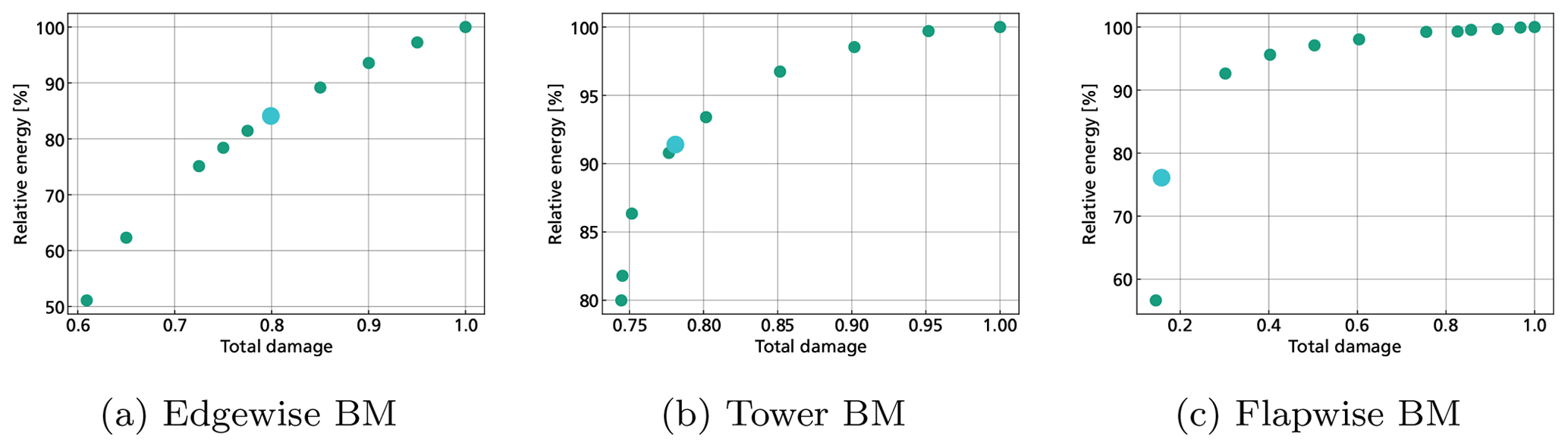
Figure 10Pareto front of relative energy production and damage for each failure mode separately.
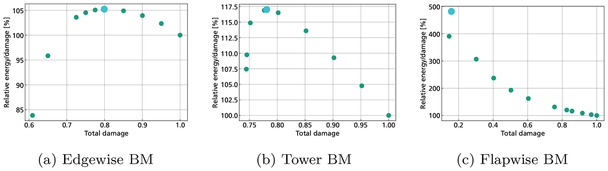
Figure 11Relative energy over damage plotted over the relative damage for each failure mode separately.
Reducing the damage results in a factor for lifetime extension, which is approximately determined by Eq. (9). According to Eq. (11), the energy yield after the extended lifetime ) is also increased by that factor. Additionally, the selected failure mode is assumed to be the only one relevant to life extension such that the damage of the others can be neglected for this example. By directly maximizing the energy production, the maximum amount of energy can be produced while fully using up the fatigue budget of the failure mode with a variable time span in this case. The result of this optimization is shown as a large blue dot in Figs. 10 and 11. Figure 11 additionally shows the relative energy production for each failure mode plotted over the relative damage. For the edgewise BM, only a slight increase in the energy production of about 5 % can be obtained when the damage is reduced between 0.75 and 0.85. For the tower BM, the reduction in damage leads to a lower loss in energy than for the edgewise BM. Therefore, the overall energy production after the extended lifetime can be significantly increased by up to 17 % when damage is reduced to 0.77. A further damage reduction reduces the effect significantly. The strongest positive effect can be seen on the flapwise BM due to the combined influence of the selected control method, the strong influence of high wind speeds and turbulence, as well as the high Wöhler exponent. The damage can be reduced to a value of 0.25 resulting in an increase in energy by more than a factor of 3. While the additional energy production for the tower BM almost increases linearly at first and then reaches the maximum value at 0.77, it clearly shows a more than linear growth for the flapwise BM. The computed Pareto fronts represent a trade-off between damage and energy production over a given time period, of which a single value and corresponding strategy need to be selected to complete the four-step process. Before we apply this step, the resulting operational strategies for each result which yields the highest relationship between energy and damage (large blue dot) are investigated more closely.
4.1.2 Detailed results of a single optimization run
To be able to interpret the optimized operational strategies, the distributions of damage with reference operation are shown for each failure mode in Fig. 12. In each plot, the wind speed is plotted radially and the wind direction circumferentially. The damage values are given by their total value share on the overall value during τlife.
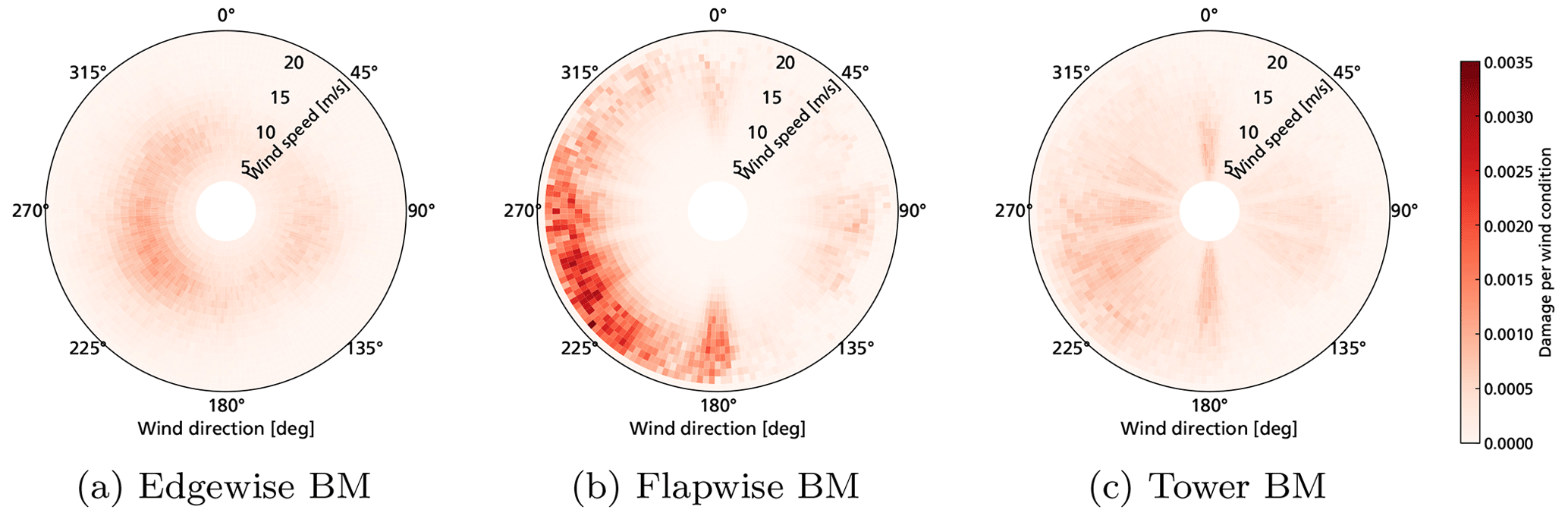
Figure 12Original distribution of damage (without applying derating) for all wind speeds (plotted radially in m s−1) and all wind directions (plotted circumferentially in degrees) of the considered turbine in the centre of the wind farm.
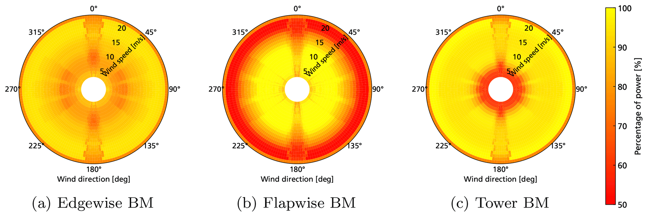
Figure 13Selection of optimized operational strategies, each of which maximizes the total relation of energy over damage for one of the failure modes. The power percentage values are plotted for all wind speeds (radially in m s−1) and directions (circumferentially in degrees).
The highest frequency in the wind distribution occurs in the southwestern direction (see Fig. 5c). This distribution is also strongly reflected in the damage value for the edgewise BM (Fig. 12a) and partially for the flapwise BM (Fig. 12b). While the highest amount of damage is induced at wind speeds below rated for the edgewise BM, the flapwise damage distribution is dominated by the high share at high wind speeds in the southwestern direction. For both, the flapwise BM and also the tower BM (Fig. 12c), there is high share of damage when they are subject to wake from the upstream surrounding turbines. The resulting operational strategies, which are optimized to reduce each of the failure modes while maximizing energy production, are shown in Fig. 13. The results depending on local wind speed and turbulence are transferred back to values depending on ambient wind speed and wind direction by sorting the results into corresponding bins. While optimization based on local wind speed and direction reduces the number of optimization variables, an implementation of the strategy based on wind direction is easier to apply in reality in an open-loop setting of the planning approach. In all three operational strategies, the reaction to the significant damage in the situations, where the turbine is in the wake of other turbines, is visible. In such situations, the damage is increased due to the wake-induced turbulence while energy production is decreased due to reduced wind speeds. This leads to a significant benefit from reducing power in such situations. In addition, each of the strategies reflects the individual behaviour of the selected failure modes and of the influence by the control setpoints under the specific conditions. While slight reduction in power, especially at low wind speeds, maximizes the energy production with the constraint on the edgewise BM (Fig. 13a), the strategy with the flapwise constraint mainly reduces power at high wind speeds (Fig. 13b). With the tower BM used as constraint, the optimized strategy selects the lowest possible setpoint of 50 % at low wind speeds up to 8 m s−1 in addition to the slight reduction in waked situations (Fig. 13c). Due to the selected method of the real-time controller, a significant load reduction can mainly be achieved at such low wind speeds for the tower. The strategies thus result overall from the interaction of the selected method and setpoints of the real-time controller, the derived surrogate models and the specified objectives of the optimizer.
4.2 Selection of best solution (step 4)
With the presented optimal planning approach, higher total energy yield can be achieved with lifetime extension, which is made possible by accepting lower annual energy production throughout the lifetime. This reduction in annual energy has a significant impact on the overall value of the wind farm, especially when taking into account economic factors that include loan repayments and the value of the money. This aspect is considered for the evaluation and selection of the operational strategies under consideration of a basic financing model. Through this first evaluation, the difference between a pure maximization of energy from the materials used and additional factors can be emphasized. We use the net present value (NPV) for this.
4.2.1 Computation of net present value
The net present value maps a future payment to its current value. We assume a constant interest rate CWACC covered by the weighted average costs of capital (WACC), constant annual maintenance costs COPEX and a constant average price of electricity CelPrice. The repayment can be variable over the entire operating period and is made depending on the annual energy yield . Currently, it is assumed to be constant in each year, because we use the same operational strategy and frequency distribution. With these parameters, the NPV can be computed for payments until a given year Y:
The future value at the end of the lifetime of an adapted operating strategy is given by NPV(Ylife) where the number of full operating years with the strategy is defined as
This model maps all future payments to their current value and thus also gives an upper bound to the initial investment that is permissible. Any revenue above the initial investment leads to additional profit.
The average costs for a wind farm are taken from BVG Associates (2019) and are summarized in Table 3. All values are scaled to a single turbine with 7.5 MW power. The financial estimations refer to an entire wind farm, so scaling it to a single turbine is not fully realistic. It can be interpreted as the “per turbine” costs of a farm. Therefore, all of these values are very rough assumptions which just allow for the possibility to compute the potential increase in profit within a realistic range.

The annual income is computed with the reference annual frequency distribution and the operational strategies from the results. An availability factor of 0.95 is assumed. In addition, we assume an electricity price of 0.064 EUR/kWh at which the wind farm is barely able to recover the investment cost after a lifetime of 25 years when being operated with the reference strategy .
4.2.2 Selection of strategy based on net present value
In Sect. 4.1.1, each of the three failure modes were considered separately. We first make a preselection of the strategy by limiting ourselves to a single failure mode. An economic evaluation is most important for tower damage. A tower replacement is usually considered to be infeasible, which in turn determines the possible lifetime of the entire wind turbine. An exchange of the rotor blade, in contrast to this, can be a feasible approach to extend the turbine's lifetime when one of its failure modes has reached its fatigue budget. Having this in mind, it is still advantageous to create a planning for these replaceable components in order to coordinate the replacement of several blades or to find the best timing. Considering all of these aspects would require further detailed models on component costs and the specific situation of a wind farm.
The financing model using the NPV from Eq. (24) is applied to all of the derating strategies which were computed for the tower in Sect. 4.1.1. The lifetime of the turbine is always determined as the time after which the induced damage has reached the fatigue budget, i.e. by Eq. (10). For the final year, the annual income is computed as a fractional value, depending on the relative damage increment before the value of 1 is reached. Here, the seasonal variations discussed in Sect. 2 are neglected.
The results are shown in Fig. 14. In all three panels, the green dashed curves correspond to the Pareto-optimal points from Fig. 10b. The blue curves highlight the one trade-off, where the maximum energy is being produced over the extended lifetime, which is almost 32 years. The light blue curves highlight the operational strategy with the best economic results, i.e. the highest NPV at the lifetime where the damage equals 1. It results in a relative damage value of 0.9 and an extended lifetime of about 27 years. Since the same frequency distribution for wind conditions and the same operating strategy is assumed for each year, also the annual damage and annual energy production are equal. This results in a linear increase in the damage in Fig. 14a and the energy production in Fig. 14b. Figure 14c shows the net present value representing the permissible investment if the system was operated until a certain year.
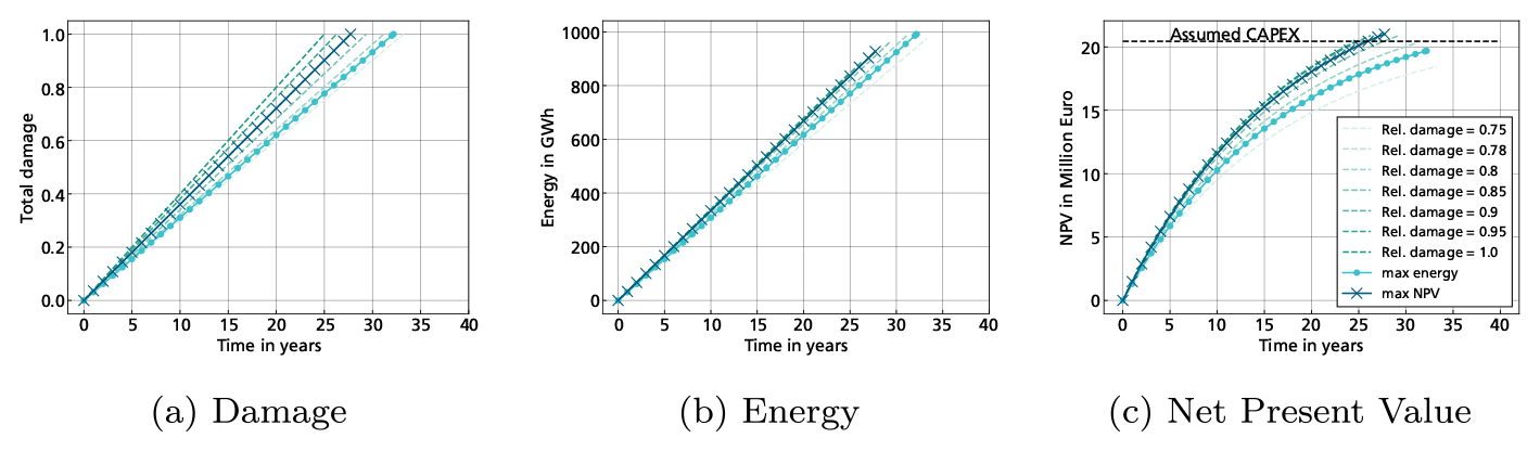
Figure 14Annual progression over time for accumulated damage, energy and NPV for multiple optimized planning strategies. Green: results of Pareto front; light blue with dots: maximum energy production; dark blue with crosses: maximum NPV).
The assumed initial costs (CAPEX) are equal to about 7.5 MW ⋅ 2.73 EUR/MW, which is ≈ EUR 20.4 million. It can be seen that for maximum energy generation, the system is not economically viable even after its extended lifetime of 32 years (cf. Fig. 14c). The NPV of that strategy is about EUR 1.7 million lower than the value with the reference strategy at 25 years. The reference strategy and the economically optimal strategy require about 25 or 26 years of operation respectively to exceed the CAPEX. The strategy which maximizes NPV is achieved with a target damage of 0.9 at a lifetime of 27 years. The difference to the reference strategy at 25 years is about EUR 0.5 million. Also, the strategies with target damages of 0.95 and 0.9 reach a higher NPV compared with the reference strategy. Therefore, these strategies will pay off after a longer operating time under the given circumstances. In contrast to this, the reduced energy yield per year of the strategy maximizing total energy (light blue curve with dots) leads to lower income, lower repayment per year and in turn to lower NPV over the entire lifetime compared with the strategy which maximizes NPV (dark blue curve with crosses) and the reference strategy (dashed dark green curve). For all strategies, it must be noted that the assumed WACC of 6 % needs to be taken into account as well. While the net present value does not change significantly in later years, the profit would increase strongly once the investment has been repaid. Thus, the actual profit can be multiplied by (1,06)r where r is the number of years operating once the investment has been returned. Therefore, a slightly higher NPV can already result in much higher profits.
Overall, the assessment of economic benefits always needs to be done under consideration of the specific assumptions and parameters for a specific project and can be done in much more detail. Especially the price of electricity underlies a high uncertainty and can hardly be predicted for 30 years in the future. Nevertheless, the exemplary evaluation shows how multiple optimized planning strategies can be used to obtain an economically optimized solution, depending on the objectives and input parameters.
The application of all four steps to the application example has shown the interaction of inputs (e.g. control setpoints), environmental conditions, damage progression, energy production and economic value. The considered example mainly illustrates that the mathematical optimization method is applicable for creating operational strategies and how the method can be used to exploit the full load-bearing capacity of one component and to increase the value of the considered system. The mathematical optimization builds on the assumptions of the underlying models and their input data. It finds the best operational strategy under these assumptions in a deterministic way. The resulting deterministic lifetime extension factor includes these assumptions and should therefore be interpreted as a potential value that needs to be validated by further assessments.
The solution also includes the uncertainties resulting either from model inaccuracies or from uncertain assumptions in the input data. This inherent limitation must always be taken into account when evaluating and discussing the results. For this reason, we have taken great care to describe the required prerequisites in detail. In addition, we have limited ourselves to the technical level first when performing the optimization (step 3). The consideration of economic factors is subject to a high degree of uncertainty due to the uncertainty of future electricity prices and other influences which are not considered. The selection of an operational strategy must always be made for a specific application, taking into account the inherent uncertainties and risk. The selection process applied in this work mainly aims at showing how the economic aspect can be taken into account and that an intelligent operational strategy can lead to higher economic profit when selected carefully.
The presented method VIOLA yields a deterministic optimal solution, which is intended as an operational plan for an uncertain future. Therefore, on the one hand, it has to be discussed how the uncertainties of the deterministic solution can be reduced by improved partial models. On the other hand, current limitations of the method and possible extensions have to be named.
5.1 Limitations and possible improvements on partial models of the current approach
The optimization process builds on the usage of surrogate models. They implement the deterministic relationship from inputs to damage and energy increments on the minutes scope. Within these models, the limits and uncertainties of various partial effects are aggregated. This includes the modelling of input conditions, the high-fidelity simulation model on the seconds scope, the calculation of damage increments and finally the selection and training of the surrogate models themselves. The modelling approach for each of these is very closely linked to the specified system boundaries.
For the application example, we have limited ourselves to two main environmental conditions and one controller setpoint as considered input conditions. These inputs define a subset and can be extended for both, environmental conditions and the possible setpoints. Fatigue damage of structural components is represented by three main failure modes. (Discussing the complexity of fatigue damage modelling goes beyond the scope of this paper; instead, readers are referred to, for example, Liao et al. (2022), which provides an overview about developments in this field.)
Regarding the environmental conditions, further influences like wind shear, yaw misalignment and wave effects for offshore wind farms can be considered. In addition, the wake effects of surrounding wind turbines can be modelled with a higher level of detail to cover effects like partial wake overlap or wake meandering. This requires an extension of the models on the minutes as well as the seconds scope.
The control setpoints of the real-time controller act as inputs to the surrogate model and as influencing variables for the optimizer. Thus, by extending the number of controller features which can be adapted and used as optimization variables, the possibilities for balancing damage under various environmental conditions increase. It would be ideal to directly optimize the control parameters under all influencing load conditions and select the trade-off according to the overall objectives, including their frequency of occurrence. Such an approach is not computationally feasible due to the need for load simulations under each condition in combination with a control parameter. Therefore, extending the possibilities of the real-time controller combined with a smart pre-selection of further control setpoints, such as allowing for partial overload or wake steering, will lead to more degrees of freedom for the long-term operational planning. With limited computational capacities, a balance between accuracy, degrees of freedom, interpretability of results and also enhancement of the approach needs to be found for specific use cases and for the optimization process itself. To assess the importance of various influences on the results, sensitivity analysis could be performed, but this is beyond the scope of this paper.
5.2 Long-term forecasting models and uncertainties
While partial models could theoretically be improved until they provide a perfect representation of reality, the forecasting over long periods of time will always be subject to remaining uncertainties. Therefore, prediction of the future always contains assumptions, which are usually modelled by a probabilistic approach. For the long-term forecast, one can distinguish between the technical part, where the forecast of environmental conditions influences the fatigue damage calculation, and the forecasting of the economic developments. This is affected by many unknowns from the global market and even politics.
Regarding the technical part, we use the classical approach for the computation of fatigue damage by covering the long-term forecast by a relative frequency distribution derived from site-specific measurements from the past. In combination with partial safety factors, such an approach is suitable for estimating a conservative design fatigue budget. Nevertheless, they neglect some important influences like annual variations of the wind (Pryor et al., 2018). Also, long-term changes in the weather due to climate change could become relevant. Hübler and Rolfes (2021) found an insignificant influence on fatigue life compared with other influences but pointed out their potential influence with improved methods. For a more detailed estimation for each individual turbine, probabilistic approaches for the fatigue damage prediction using surrogate models can be used, e.g. by using Monte Carlo simulations with a representative time series (Hübler, 2019) or by using stochastic distributions for modelling the uncertainty (Nielsen et al., 2021). Due to the high computational effort, such approaches are less suitable for the use within an optimization loop. The probabilistic approach for fatigue life prediction is strongly connected with the choice of inputs for the models. One also needs to distinguish between conditions which can be influenced by control setpoints of the controller, and conditions which cannot be influenced (e.g. idling) but which nevertheless contribute to the overall damage process. Therefore, it is also possible to reduce uncertainties with further details in the models. To determine the overall risk, it is required to assess the uncertainties of the partial models and the forecasts.
In our current implementation of the proposed method, a very basic approach for the financial part, i.e. computing the asset value, is implemented. Regulatory and legal framework conditions are excluded from the model, as they can change over time and are strongly dependent on the specific location. Also, our focus is on showing the technical feasibility. Covering all regulatory aspects and expected, planned or coming legislation is a highly specialized but separate task. Nevertheless, the current approach can be supplemented with further inputs to reduce the uncertainties. Also, other value metrics, such as the cost of valued energy (COVE), could be integrated (Loth et al., 2022). A highly significant influence is the price of electricity, which is not constant over the entire lifetime.
In summary, the amount of detail in the mathematical optimization process has to be a deliberate decision. This decision also depends on other parameters like the available computational power and the optimization method. With the current subdivision into two parts – the technical, deterministic optimization in step 3 and the subsequent selection based on additional (economic) factors in step 4 – the mathematical optimization problem can be solved with low computational effort, and the deterministic solutions are well understandable and interpretable. Nevertheless, several drawbacks to our approach remain and are discussed next.
5.3 Limitations and potential improvements of the optimization method VIOLA
Without any limitations on computational power and time, the robust optimization approach which directly maximizes the asset value as an objective containing further inputs like, for example, reliability models, component replacement costs and forecasts of the market, including their probabilistic uncertainties, would be ideal. To approach such an ideal solution within given boundaries, several smaller steps can be made.
The deterministic optimization method is currently limited to a single turbine. The influence of the turbine controller on the wake and thus on surrounding turbines is neglected. To extend our approach to an entire wind farm two possible solutions exist. The first way is to optimize operation of all turbines once, but this could increase the size of the optimization problem beyond feasibility. The second solution could be to iteratively cycle through computing inflow conditions for an individual turbine from a wind farm flow model and then optimize operation for each turbine separately for their respective inflow conditions. We expect such an approach to converge after a few cycles while keeping computational requirements at bay and scaling well. Both solutions allow a combination with farm control solutions, such as wake steering.
Overall, any deterministic solution of a single turbine or an entire wind farm requires the specification of an individual target damage for each selected failure mode. Here, the specification of a desired target reliability level for the components of each wind turbine could be covered by probabilistic reliability methods. Further research is required to assess how this can be integrated with the current method. It also needs to be investigated how the computation of any value metric can be integrated into the optimization approach, either directly within the mathematical optimization or for a subsequent selection of Pareto-optimal operational strategies.
To cover the forecast of volatile market prices within the deterministic mathematical optimization, the annual frequency distribution of input conditions can be extended with another dimension for price and thus a combined probability for wind and price, similar to the approach in Loepelmann and Fischer (2022). In addition, an annual selection of the trade-off between energy and damage could be integrated into the optimization. This way, it would be possible to allow for a higher damage progression at the beginning to reduce the interest burden and to reduce the damage progression of the turbine later.
One aspect, which cannot be covered by the current planning approach, is considering sequence effects, i.e. dependencies of future damage progression on previous damage. With the use of frequency distributions for long-term effects, linearity of damage progression is inherently assumed. To consider sequence effects, the current approach can at least be used as an initial planning step, partially covering the linear part of a damage progression process.
5.4 Application of optimized strategies
Regardless of the limitations, the results of the application example show how a condition-based long-term planning approach can realize a targeted fatigue damage progression. It balances the trade-off between induced damage and energy production under the given system boundaries and constraints of the application example optimally. It is possible to apply the method to a real-world scenario when the system boundaries are well defined and adapted to the specific use case. In a first step, the provided planning strategy can be used in an open-loop scenario, where the turbine follows the planned setpoints. The open-loop approach can also be used to extend the lifetime after the turbine has already been operating for a significant time span. If the approach is applied during the design process, it could be used to save material through a less conservative design or to optimize the power curve as part of the real-time controller. In a second step, the approach could be further developed into reliability-adaptive control, where measurements of turbine operation are fed back into continuous re-planning, thus forming a closed-loop controller as presented on the right side of Fig. 1.
We presented a novel method for an optimal planning for the operation of wind energy systems over their entire lifetime. This comprises a four-step process, of which the key is to formulate a mathematical optimization problem which optimally distributes the available damage budget of a given failure mode over the total turbine lifetime. In the introduction, the objectives for this work were derived from the context of reliability(-adaptive) control. A planning, which pursues long-term objectives of operation, was identified as an important input. Our process is focused on the planning of the fatigue damage progression of different wind turbine failure modes. As a basis, the theoretical background for the deterministic computation of fatigue damage progression was introduced. The process is applied to an application example for demonstration, which serves as a proof of concept.
Each of the four steps is introduced providing some general background and subsequently applied to the demonstration example. Tho process starts by providing setpoints for the real-time controller of a wind turbine (step 1) and is continued by their usage as an input for the creation of surrogate models for the induced damage (step 2). Those two steps were identified as required prerequisites for the new method VIOLA consisting of steps 3 and 4. In step 3, the mathematical nonlinear optimization problem is developed and solved using the surrogates from step 2. Several Pareto-optimal operational strategies are found as results. Finally, the results are selected based on an economic evaluation (step 4). The application example shows the great potential for an effective planning of damage progression in relation to energy production. By assessing several strategies based on the economic value, the potential and risk of such strategies become apparent at the same time. Many of the limitations, assumptions and potential improvements were discussed in Sect. 5. The key is to use partial models within their assumptions and limitations. They must be carefully examined and tested for each actual use case. Improvements, starting from the real-time controller, over the damage calculation with surrogates up to long-term predictions, can be made in the respective domain.
In our future work, we want to focus on further development of the method VIOLA. Here, one can distinguish between further improvement of the currently used deterministic mathematical optimization and the use of probabilistic methods. For the deterministic part, a first step would be an extension of the system boundaries for the operational planning of all turbines in a wind farm at once. In addition, operational strategies need to be able to handle volatile market prices and further requirements of future wind energy systems. This could be combined with control setpoints for uprating or power boost and for grid support. With all these aspects, we aim at integrating wind farm flow control considering electricity prices, as shown in Kölle et al. (2022a), with our optimal planning of the damage progression to increase the value of wind farms. Since the deterministic approach for fatigue damage progression neglects the stochastic nature of system and component failures, probabilistic approaches to define target reliability values for each wind turbine as a system can be employed. At first, probabilistic approaches can be used for the selection of the best operational strategy by estimating the underlying uncertainty. Subsequently, it needs to be evaluated if and how the uncertainty assessment can be integrated into the optimization process, e.g. using robust optimization methods. Stochastic methods can also be applied to integrate the uncertainties of the future market.
To apply the strategy during operation, coupling the planning stage with the operational stage is required. As a first step, open-loop control can be implemented. To do so, the properties of a specific wind turbine or wind farm need to be identified and coupled with the planning approach. Regular readjustment of the planning, as also indicated in Fig. 1, would allow for a simplified semi-continuous adaption of the system based on current system performance. In such a scenario, it needs to be examined how short-term deviations from the planning, for example, by reacting on electricity prices or simply on grid requirements, can be tolerated while at the same time following the provided planning sufficiently well. The best time and way to readjust the planning also need to be investigated. Connecting the operational planning with additional inputs like maintenance planning would bring further advantageous to the approach. Real closed-loop behaviour, where the planning provides setpoints for a reliability controller, has an even higher overall potential but also brings further challenges which were discussed in the introduction (Sect. 1.1).
In the future, the coupled operation of wind turbines or wind farms with power-to-X systems will become highly relevant. This increases the need for adaptive operation because the damage progression of connected systems also needs to be considered, and the question of when to operate each system, and on what level, needs to be answered. Therefore, such a coupled operation leads to a further expansion of the system boundaries and brings more complexity on different levels. For hydrogen production, the damage progression in electrolyzers needs to be integrated in order to assess their reliability. It is also necessary to include prices for selling hydrogen, and thus to serve a second market.
In conclusion, the presented work provides an applicable and adaptable method for the long-term planning of wind turbine operation. More research is needed to reduce uncertainty and consider multiple components and failure modes in the planning. Additionally, the integration with reliability-adaptive control offers further advancements to discover the full benefits for a more sustainable wind farm operation.
| fm: | failure mode |
| : | reference operational strategy |
| τref: | reference lifetime |
| : | optimized operational strategy |
| : | arbitrary operational strategy |
| τlife: | free modified lifetime |
| Δτ: | time increment for long-term planning, |
| e.g. 1 year | |
| Y: | number of time increments |
| cext: | extension factor |
| ): | extension factor for failure mode fm |
| depending on operational strategy | |
| ): | chosen operation period for failure mode |
| fm depending on operational strategy | |
| Δt: | time increment for the definition of input |
| condition, e.g. 1 h | |
| x∈X: | external input conditions valid for a |
| time of Δt | |
| : | set of input conditions with Bx bins |
| Bx: | number of bins for all input conditions |
| xj: | input conditions for bin j |
| w=Dim(X): | number of independent wind conditions |
| : | number of bins defined for condition x(i) |
| u(x)∈U: | setpoints for real-time controller |
| depending on x | |
| : | definition for operational strategy as set |
| of setpoints depending on | |
| pΔτ(x): | relative frequency distribution of |
| input conditions | |
| hτ(x): | absolute frequency distribution of input |
| conditions for a time period τ | |
| href: | reference absolute frequency distribution |
| which is applied for planning of a site | |
| ): | function for damage for a failure mode |
| with variable τ depending on the | |
| operating strategy and the frequency | |
| distribution as parameters | |
| ): | annual or mean damage for strategy |
| (time period Δτ) | |
| dfm(x,u): | damage increment for failure mode |
| (time increment Δt) | |
| P(x,u): | energy increment under the input |
| conditions (time increment Δt) | |
| ): | function for energy production with |
| variable τ depending on the operating | |
| strategy and the frequency distribution | |
| as parameters | |
| ): | annual or mean energy for strategy |
| (time period Δτ) |
| ni: | number of load cycles |
| Ni: | maximum bearable number of load cycles |
| Dult: | ultimate design load |
| m: | Wöhler coefficient |
| Lij: | oscillation amplitude of a load cycle |
| Neq: | number of equivalent load cycles |
| DELst(x,u): | short-term damage equivalent load |
| ): | lifetime damage equivalent load |
| DELref: | reference damage equivalent load |
| ): | input to surrogate model as a |
| combination of external conditions and | |
| control setpoints | |
| ): | input sampling for the creation of |
| surrogate models | |
| fDEL(z): | surrogate function for DEL of |
| failure mode | |
| fP(z): | surrogate function for power production |
| : | target fatigue budget for failure mode |
| NPV(Y): | net present value depending on year Y |
| CelPrice: | constant electricity price |
| COPEX: | constant annual costs for operation |
| and maintenance | |
| cWACC: | constant interest rate defined as weighted |
| average costs of capital (WACC) | |
| vamb: | ambient wind speed |
| v: | local wind speed |
| TI: | local turbulence intensity |
| θamb: | ambient wind direction |
| s: | turbine index in a wind farm |
| S: | number of turbines in a wind farm |
| ): | wake calculation function for a turbine s |
| Bv: | number of bins for local wind speed |
| BTI: | number of bins for local turbulence |
| intensity | |
| M: | generator torque |
| k: | generator torque coefficient |
| Mr: | rated generator torque |
| ωr: | rated generator speed |
| δP: | percentage power factor |
| β: | pitch angle |
| λ: | tip speed ratio |
| Pr: | rated power |
| δω: | percentage generator speed factor |
Codes and data were created for each step of the published method. However, some of the tools used are very specific to an in-house workflow and are only partially documented. Thus, there is no single self-contained program of which sharing would provide value for others. The dataset of short-term DELs, used to create the surrogate models, can be found at https://doi.org/10.5281/zenodo.8385296 (Requate and Meyer, 2023). For inquiries about data or code, please contact the authors.
NR and TM developed the concept for the study and the research methods. NR developed the code and produced the results under supervision and with valuable input from TM. TM was responsible for project administration and funding acquisition. NR wrote the draft version of the paper. RH reviewed the draft version and gave valuable feedback on the draft, the concept and the results. TM and NR reviewed and edited the draft version.
The contact author has declared that none of the authors has any competing interests.
Publisher’s note: Copernicus Publications remains neutral with regard to jurisdictional claims made in the text, published maps, institutional affiliations, or any other geographical representation in this paper. While Copernicus Publications makes every effort to include appropriate place names, the final responsibility lies with the authors.
We thank Vasilils Pettas for the publicly attributed review and for the fruitful discussions that followed.
The research was carried out by Fraunhofer IWES under the framework of two research projects funded by the Bundesministerium für Bildung und Forschung (BMBF): H2-DIGITAL (grant no. 03SF0635) and Verbundvorhaben H2Mare_VB0: OffgridWind (grant no. 03HY300E). Additionally, parts of the work were conducted within the project DigiWind in cooperation with TU Wien. TU Wien was funded by VGB Powertech e.V. in DigiWind.
This paper was edited by Jennifer King and reviewed by Vasilis Pettas and one anonymous referee.
Andersson, L. E., Anaya-Lara, O., Tande, J. O., Merz, K. O., and Imsland, L.: Wind farm control – Part I: A review on control system concepts and structures, IET Renew. Power Gen., 37, 1703, https://doi.org/10.1049/rpg2.12160, 2021. a
Astrain Juangarcia, D., Eguinoa, I., and Knudsen, T.: Derating a single wind farm turbine for reducing its wake and fatigue, J. Phys. Conf. Ser., 1037, 032039, https://doi.org/10.1088/1742-6596/1037/3/032039, 2018. a
Bastankhah, M. and Porté-Agel, F.: Experimental and theoretical study of wind turbine wakes in yawed conditions, J. Fluid Mech., 806, 506–541, https://doi.org/10.1017/jfm.2016.595, 2016. a
Bech, J. I., Hasager, C. B., and Bak, C.: Extending the life of wind turbine blade leading edges by reducing the tip speed during extreme precipitation events, Wind Energ. Sci., 3, 729–748, https://doi.org/10.5194/wes-3-729-2018, 2018. a
Beganovic, N. and Söffker, D.: Structural health management utilization for lifetime prognosis and advanced control strategy deployment of wind turbines: An overview and outlook concerning actual methods, tools, and obtained results, Renew. Sust. Energ. Rev., 64, 68–83, https://doi.org/10.1016/j.rser.2016.05.083, 2016. a
Biscani, F. and Izzo, D.: pygmo, https://esa.github.io/pygmo2/index.html (last access: 3 November 2023), 2020a. a
Biscani, F. and Izzo, D.: A parallel global multiobjective framework for optimization: pagmo, Journal of Open Source Software, 5, 2338, https://doi.org/10.21105/joss.02338, 2020b. a
Bossanyi, E.: Combining induction control and wake steering for wind farm energy and fatigue loads optimisation, J. Phys. Conf. Ser., 1037, 032011, https://doi.org/10.1088/1742-6596/1037/3/032011, 2018. a
Bossanyi, E. and Jorge, T.: Optimisation of wind plant sector management for energy and loads, in: 2016 European Control Conference (ECC), IEEE, Piscataway, NJ, 922–927, https://doi.org/10.1109/ECC.2016.7810407, 2016. a
Burton, T., Jenkins, N., Sharpe, D., and Bossanyi, E.: Wind Energy Handbook, John Wiley & Sons, Hoboken, 2 edn., https://doi.org/10.1002/9781119992714, 2011. a
BVG Associates: Wind farm costs – Guide to an offshore wind farm, https://guidetoanoffshorewindfarm.com/wind-farm-costs (last access: 3 November 2023), 2019. a
Chiandussi, G., Codegone, M., Ferrero, S., and Varesio, F. E.: Comparison of multi-objective optimization methodologies for engineering applications, Comput. Math. Appl., 63, 912–942, https://doi.org/10.1016/j.camwa.2011.11.057, 2012. a
Debusscher, C. M. J., Göçmen, T., and Andersen, S. J.: Probabilistic surrogates for flow control using combined control strategies, J. Phys. Conf. Ser., 2265, 032110, https://doi.org/10.1088/1742-6596/2265/3/032110, 2022. a
Dimitrov, N.: Surrogate models for parameterized representation of wake–induced loads in wind farms, Wind Energy, 22, 1371–1389, https://doi.org/10.1002/we.2362, 2019. a, b
Dimitrov, N., Kelly, M. C., Vignaroli, A., and Berg, J.: From wind to loads: wind turbine site-specific load estimation with surrogate models trained on high-fidelity load databases, Wind Energ. Sci., 3, 767–790, https://doi.org/10.5194/wes-3-767-2018, 2018. a
DNVGL-ST-0263: Certification of lifetime extension of wind turbines, Standard, 2016. a
Do, M. H. and Söffker, D.: State-of-the-art in integrated prognostics and health management control for utility-scale wind turbines, Renew. Sust. Energ. Rev., 145, 111102, https://doi.org/10.1016/j.rser.2021.111102, 2021. a
Eguinoa, I., Göçmen, T., Garcia-Rosa, P. B., Das, K., Petrović, V., Kölle, K., Manjock, A., Koivisto, M. J., and Smailes, M.: Wind farm flow control oriented to electricity markets and grid integration: Initial perspective analysis, Advanced Control for Applications, 3, 1–28, https://doi.org/10.1002/adc2.80, 2021. a
Elorza, I., Calleja, C., and Pujana-Arrese, A.: On Wind Turbine Power Delta Control, Energies, 12, 2344, https://doi.org/10.3390/en12122344, 2019. a
Fleming, P. A., Aho, J., Buckspan, A., Ela, E., Zhang, Y., Gevorgian, V., Scholbrock, A., Pao, L., and Damiani, R.: Effects of power reserve control on wind turbine structural loading, Wind Energy, 19, 453–469, https://doi.org/10.1002/we.1844, 2016. a
Gasparis, G., Lio, W. H., and Meng, F.: Surrogate Models for Wind Turbine Electrical Power and Fatigue Loads in Wind Farm, Energies, 13, 6360, https://doi.org/10.3390/en13236360, 2020. a
Harrison, M., Bossanyi, E., Ruisi, R., and Skeen, N.: An initial study into the potential of wind farm control to reduce fatigue loads and extend asset life, J. Phys. Conf. Ser., 1618, 022007, https://doi.org/10.1088/1742-6596/1618/2/022007, 2020. a
Hersbach, H., Bell, B., Berrisford, P., Biavati, G., Horányi, A., Muñoz Sabater, J., Nicolas, J., Peubey, C., Radu, R., Rozum, I., Schepers, D., Simmons, A., Soci, C., Dee, D., and Thépaut, J.-N.: ERA5 hourly data on single levels from 1959 to present, CDS [data set], https://doi.org/10.24381/cds.adbb2d47, 2018. a
Houck, D. R.: Review of wake management techniques for wind turbines, Wind Energy, 25, 195–220, https://doi.org/10.1002/we.2668, 2022. a, b, c
Hübler, C. and Rolfes, R.: Analysis of the influence of climate change on the fatigue lifetime of offshore wind turbines using imprecise probabilities, Wind Energy, 24, 275–289, https://doi.org/10.1002/we.2572, 2021. a
Hübler, C. J.: Efficient probabilistic analysis of offshore wind turbines based on time-domain simulations, Dissertation, Gottfried Wilhelm Leibniz Universität, Hannover, https://doi.org/10.15488/4822, 2019. a, b
IEC: Wind Turbines – Part 1: Design Requirements, IEC 61400-1, International Standard, 2019. a, b, c, d
Jonkman, B. J.: TurbSim User's Guide: Version 1.50, NREL, https://doi.org/10.2172/965520, 2009. a
Kanev, S., Bot, E., and Giles, J.: Wind Farm Loads under Wake Redirection Control, Energies, 13, 4088, https://doi.org/10.3390/en13164088, 2020. a
Kanev, S. K., Savenije, F. J., and Engels, W. P.: Active wake control: An approach to optimize the lifetime operation of wind farms, Wind Energy, 21, 488–501, https://doi.org/10.1002/we.2173, 2018. a
Kölle, K., Göçmen, T., Eguinoa, I., Alcayaga Román, L. A., Aparicio-Sanchez, M., Feng, J., Meyers, J., Pettas, V., and Sood, I.: FarmConners market showcase results: wind farm flow control considering electricity prices, Wind Energ. Sci., 7, 2181–2200, https://doi.org/10.5194/wes-7-2181-2022, 2022a. a, b
Kölle, K., Göçmen, T., Garcia-Rosa, P. B., Petrović, V., Eguinoa, I., Vrana, T. K., Long, Q., Pettas, V., Anand, A., Barlas, T. K., Cutululis, N., Manjock, A., Tande, J. O., Ruisi, R., and Bossanyi, E.: Towards integrated wind farm control: interfacing farm flow and power plant controls, Advanced Control for Applications, 4, e105, https://doi.org/10.1002/adc2.105, 2022b. a
Leimeister, M. and Thomas, P.: The OneWind Modelica Library for Floating Offshore Wind Turbine Simulations with Flexible Structures, in: Proceedings of the 12th International Modelica Conference, edited by: Kofránek, J. and Casella, F., Modelica Association and Linköping University Electronic Press, Linköping, 633–642, https://doi.org/10.3384/ecp17132633, 2017. a
Liao, D., Zhu, S.-P., Correia, J. A., de Jesus, A. M., Veljkovic, M., and Berto, F.: Fatigue reliability of wind turbines: historical perspectives, recent developments and future prospects, Renew. Energ., 200, 724–742, https://doi.org/10.1016/j.renene.2022.09.093, 2022. a
Loepelmann, P. and Fischer, B.: Lifetime extension and opex reduction by adapting the operational strategy of wind farms, J. Phys. Conf. Ser., 2257, 012014, https://doi.org/10.1088/1742-6596/2257/1/012014, 2022. a
Loew, S., Obradovic, D., and Bottasso, C. L.: Model predictive control of wind turbine fatigue via online rainflow-counting on stress history and prediction, J. Phys. Conf. Ser., 1618, 022041, https://doi.org/10.1088/1742-6596/1618/2/022041, 2020. a
Lorenzo, C. F. and Merrill, W. C.: Life Extending Control – A Concept Paper, in: American Control Conference, 1991, IEEE, Piscataway, 1081–1095, https://doi.org/10.23919/ACC.1991.4791545, 1991. a
Loth, E., Qin, C., Simpson, J. G., and Dykes, K.: Why we must move beyond LCOE for renewable energy design, Advances in Applied Energy, 8, 100112, https://doi.org/10.1016/j.adapen.2022.100112, 2022. a
Mendez Reyes, H., Kanev, S., Doekemeijer, B., and van Wingerden, J.-W.: Validation of a lookup-table approach to modeling turbine fatigue loads in wind farms under active wake control, Wind Energ. Sci., 4, 549–561, https://doi.org/10.5194/wes-4-549-2019, 2019. a
Meyer, T.: Optimization-based reliability control of mechatronic systems, Ph.D. Thesis, Universität Paderborn, https://doi.org/10.17619/UNIPB/1-3, 2016. a
Meyer, T., Fischer, K., Wenske, J., and Reuter, A.: Closed-loop supervisory control for defined component reliability levels and optimized power generation, in: Windeurope Conference and Exhibition Proceedings, https://doi.org/10.24406/publica-fhg-406740, 2017. a
Meyers, J., Bottasso, C., Dykes, K., Fleming, P., Gebraad, P., Giebel, G., Göçmen, T., and van Wingerden, J.-W.: Wind farm flow control: prospects and challenges, Wind Energ. Sci., 7, 2271–2306, https://doi.org/10.5194/wes-7-2271-2022, 2022. a, b
Miner, M. A.: Cumulative Damage in Fatigue, J. Appl. Mech., 12, A159–A164, https://doi.org/10.1115/1.4009458, 1945. a
Mozafari, S., Dykes, K., Rinker, J. M., and Veers, P.: Effects of finite sampling on fatigue damage estimation of wind turbine components: A statistical study, Wind Engineering, 47, 0309524X2311638, https://doi.org/10.1177/0309524X231163825, 2023. a
Nash, R., Nouri, R., and Vasel-Be-Hagh, A.: Wind turbine wake control strategies: A review and concept proposal, Energ. Convers. Manage., 245, 114581, https://doi.org/10.1016/j.enconman.2021.114581, 2021. a, b, c
Nielsen, J. S., Miller-Branovacki, L., and Carriveau, R.: Probabilistic and Risk-Informed Life Extension Assessment of Wind Turbine Structural Components, Energies, 14, 821, https://doi.org/10.3390/en14040821, 2021. a
Njiri, J. G. and Söffker, D.: State-of-the-art in wind turbine control: Trends and challenges, Renew. Sust. Energ. Rev., 60, 377–393, https://doi.org/10.1016/j.rser.2016.01.110, 2016. a
Njiri, J. G., Beganovic, N., Do, M. H., and Söffker, D.: Consideration of lifetime and fatigue load in wind turbine control, Renew. Energ., 131, 818–828, https://doi.org/10.1016/j.renene.2018.07.109, 2019. a
Pettas, V. and Cheng, P. W.: Down-regulation and individual blade control as lifetime extension enablers, J. Phys. Conf. Ser., 1102, 012026, https://doi.org/10.1088/1742-6596/1102/1/012026, 2018. a
Pettas, V., Salari, M., Schlipf, D., and Cheng, P. W.: Investigation on the potential of individual blade control for lifetime extension, J. Phys. Conf. Ser., 1037, 032006, https://doi.org/10.1088/1742-6596/1037/3/032006, 2018. a, b
Popko, W., Thomas, P., Sevinc, A., Rosemeier, M., Bätge, M., Braun, R., Meng, F., Horte, D., and Balzani, C.: IWES Wind Turbine IWT-7.5-164. Rev 4, Fraunhofer IWES, Bremerhaven, https://doi.org/10.24406/IWES-N-518562, 2018. a
Pryor, S. C., Shepherd, T. J., and Barthelmie, R. J.: Interannual variability of wind climates and wind turbine annual energy production, Wind Energ. Sci., 3, 651–665, https://doi.org/10.5194/wes-3-651-2018, 2018. a
Rakowsky, K. U.: An introduction to Reliability-Adaptive Systems, in: Advances in Safety and Reliability, edited by: Kolowrocki, K., 1633–1636, ISBN 0415383404, 2005. a
Rakowsky, U. K.: Modelling Reliability-Adaptive multi-system operation, International Journal of Automation and Computing, 3, 192–198, https://doi.org/10.1007/s11633-006-0192-8, 2006. a
Requate, N. and Meyer, T.: Active Control of the Reliability of Wind Turbines, IFAC-PapersOnLine, 53, 12789–12796, https://doi.org/10.1016/j.ifacol.2020.12.1941, 2020. a, b
Requate, N. and Meyer, T.: Database of Short Term Damage Equivalent Loads (DEL) of IWT7.5MW wind turbine depending on wind, TI, yaw and derating, Zenodo [data set], https://doi.org/10.5281/zenodo.8385296, 2023. a
Requate, N., Wiens, M., and Meyer, T.: A Structured Wind Turbine Controller Evaluation Process Embedded into the V-Model for System Development, J. Phys. Conf. Ser., 1618, 022045, https://doi.org/10.1088/1742-6596/1618/2/022045, 2020. a
Santos, R. A.: Damage mitigating control for wind turbines, Ph.D. Thesis, The University of Colorado, Colorado, 2006. a
Santos, R. A.: Control system for wind turbine (U.S Patent No. US20080086281A1), https://worldwide.espacenet.com/publicationDetails/biblio?FT=D&CC=US&NR=2008086281A1&KC=A1 (last access: 3 November 2023), 2008. a
Schmidt, J.: FOXES (Farm Optimization and eXtended yield Evaluation Software), https://fraunhoferiwes.github.io/foxes.docs/index.html (last access: 3 November 2023), 2022. a
Schmidt, J., Requate, N., and Vollmer, L.: Wind Farm Yield and Lifetime Optimization by Smart Steering of Wakes, J. Phys. Conf. Ser., 1934, 012020, https://doi.org/10.1088/1742-6596/1934/1/012020, 2021. a
Singh, D., Dwight, R. P., Laugesen, K., Beaudet, L., and Viré, A.: Probabilistic surrogate modeling of offshore wind-turbine loads with chained Gaussian processes, J. Phys. Conf. Ser., 2265, 032070, https://doi.org/10.1088/1742-6596/2265/3/032070, 2022. a
Slot, R. M., Sørensen, J. D., Sudret, B., Svenningsen, L., and Thøgersen, M. L.: Surrogate model uncertainty in wind turbine reliability assessment, Renew. Energ., 151, 1150–1162, https://doi.org/10.1016/j.renene.2019.11.101, 2020. a
Söffker, D. and Rakowsky, U. K.: Perspectives of monitoring and control of vibrating structures by combining new methods of fault detection with new approaches of reliability engineering, A Critical Link: Diagnosis to Prognosis, 671–682, 1997. a
Sutherland, H. J.: On the Fatigue Analysis of Wind Turbines, Sandia National Labs., Albuquerque, NM (US), Sandia National Laboratories, Albuquerque, New Mexico, https://doi.org/10.2172/9460, 1999. a, b
Thomas, P.: MoWiT, http://www.mowit.info (last access: 3 November 2023), 2022. a
Thomas, P., Gu, X., Samlaus, R., Hillmann, C., and Wihlfahrt, U.: The OneWind Modelica Library for Wind Turbine Simulation with Flexible Structure – Modal Reduction Method in Modelica, in: Proceedings of the 10th International Modelica Conference, Linköping Electronic Conference Proceedings, Linköping University Electronic Press, 939–948, https://doi.org/10.3384/ecp14096939, 2014. a
van der Hoek, D., Kanev, S., and Engels, W.: Comparison of Down-Regulation Strategies for Wind Farm Control and their Effects on Fatigue Loads, in: 2018 Annual American Control Conference (ACC), IEEE, 3116–3121, https://doi.org/10.23919/ACC.2018.8431162, 2018. a, b, c
Waechter, A. and Laird, C.: Ipopt, https://coin-or.github.io/Ipopt/index.html (last access: 3 November 2023), 2022. a
Wiens, M.: Turbine operation: Control systems keep everything running smoothly, https://websites.fraunhofer.de/IWES-Blog/en/turbine-operation-control-systems-keep-everything-running-smoothly/marcus-wiens (last access: 3 November 2023), 2021. a
In general, there are various terms for reducing the power of a wind turbine and the usage often depends on the context. In wind farm control, the term “axial-induction control” is often used. Also, “down-regulation” or “curtailment” are prominent terms. The latter term is often referred to in the context of requests by the grid operator. The term “derating” is used throughout this work.
Note that in our notation we distinguish between inputs and parameters of the defined function. Parameters are assumed to be fixed for a specific use case. They are separated by a semicolon, whereas the function inputs are in front of the semicolon. If additional parameters exist but are not important for a certain passage, we omit them to improve readability and replace them with a centred dot (⋅). So for ), τref is an input, is a set of parameters and ⋅ denotes that additional parameters are omitted.
- Abstract
- Introduction
- Theoretical background
- Definition of example system and implementing prerequisites for optimization
- Method for optimal long-term planning: VIOLA
- Discussion
- Conclusion and Outlook
- Appendix A: List of symbols
- Code and data availability
- Author contributions
- Competing interests
- Disclaimer
- Acknowledgements
- Financial support
- Review statement
- References