Quantification and correction of motion influence for nacelle-based lidar systems on floating wind turbines

Inflow wind field measurements from nacelle-based lidar systems offer great potential for different applications including turbine control, load validation, and power performance measurements. On floating wind turbines nacelle-based lidar measurements are affected by the dynamic behavior of the floating foundations. Therefore, the effects on lidar wind speed measurements induced by floater dynamics must be understood. In this work, we investigate the influence of floater motions on wind speed measurements from forward-looking nacelle-based lidar systems mounted on floating offshore wind turbines (FOWTs) and suggest approaches for correcting motion-induced effects. We use an analytical model, employing the guide for the expression of uncertainty in measurements (GUM) methodology and a numerical lidar simulation for the quantification of uncertainties. It is found that the uncertainty of lidar wind speed estimates is mainly caused by the fore–aft motion of the lidar, resulting from the pitch displacement of the floater. Therefore, the uncertainty is heavily dependent on the amplitude and the frequency of the pitch motion. The bias of 10 min mean wind speed estimates is mainly influenced by the mean pitch angle of the floater and the pitch amplitude. We correct motion-induced biases in time-averaged lidar wind speed measurements with a model-based approach, employing the developed analytical model for uncertainty and bias quantification. Testing of the approach with simulated dynamics from two different FOWT concepts shows good results with remaining mean errors below 0.1 m s⁻¹. For the correction of motion-induced fluctuation in instantaneous measurements, we use a frequency filter to correct fluctuations caused by floater pitch motions for instantaneous measurements. The correction approach's performance depends on the pitch period and amplitude of the FOWT design.

1 Introduction

With many countries worldwide having ambitious targets for FOWT installations and a pipeline of upcoming projects, the installed capacity of FOWT is expected to increase exponentially in the coming decade. Forecasts expect the global installed capacity of floating wind to reach 16.5 GW by 2030 (GWEC, 2022). While FOWTs offer the potential to exploit wind resources in deep waters, new challenges occur due to the dynamic behavior of floating support structures. One of these challenges is the reliable measurement of wind resources and FOWT inflow conditions.

For wind measurements in deep waters, typically met masts are not applicable due to high installation costs. As an alternative, floating lidar concepts have been developed and are already used in industry projects and research applications. A comprehensive overview of the technology and challenges can be found in Gottschall et al. (2017). The use of forward-looking nacelle-based lidar systems is advantageous to measure inflow conditions to individual turbines. Potential use cases for nacelle-based lidar systems include power performance monitoring, load monitoring, and turbine control.

Özinan et al. (2022) published a power curve assessment campaign with a nacelle-based lidar on a 2 MW FOWT. This study compared lidar measurements to a nacelle-mounted sonic anemometer. While a good agreement between both wind speed references was observed, the power curves with lidar wind speed measurements showed higher scatter compared to the nacelle cup-anemometer measurements. It can be expected that the increased scatter is caused by the influence of floater dynamics and the corresponding shift of the measurement position on lidar measurements. However, no systematic analysis and quantification of motion-induced effects are presented in this study.

In Conti et al. (2020) load simulations have been performed using lidar-estimated wind field characteristics (WFCs). Predicted loads have been compared to load measurements at the turbine. In Conti et al. (2021) a methodology for combining nacelle-based lidar measurements with constrained wind field reconstruction techniques has been proposed to improve the accuracy of load assessments for fixed-bottom wind turbines. Since this study was performed for bottom-fixed wind turbines, no effects of floating dynamics are considered. The effect of floater dynamics on measured wind speed time series must be investigated to transfer the proposed methodology to the case of floating wind turbines.

Another application of nacelle-based lidar systems is the use of different lidar-assisted wind turbine control strategies. These control strategies aim to use knowledge about the approaching wind field to optimize the operation of the turbine. Investigated concepts include collective and individual pitch control (see, e.g., Bossanyi et al., 2014), yaw control (see, e.g., Fleming et al., 2014), and speed control (see, e.g., Schlipf et al., 2013). The abovementioned studies did not investigate the proposed control strategies for floating wind turbines and did not consider the effect of floater dynamics on the inflow measurements used.

Although different applications require wind speed measurements in different temporal resolutions (e.g., 1 Hz for turbine control versus 10 min average for performance measurements), for all the abovementioned applications the quantification of uncertainties and biases in lidar measurements is essential. The need for uncertainty quantification and the development of suitable tools and models has also been highlighted as an important step towards the broad application of nacelle-based lidar systems by Clifton et al. (2018).

While the abovementioned studies have mainly investigated the use of nacelle-based lidar systems for the measurement of inflow conditions of onshore or bottom-fixed offshore wind turbines, little experience exists for the use on FOWT. Since the floating dynamics of the FOWT causes translational and rotational displacement of nacelle-mounted lidars, it can be expected that these dynamics affect the measurements. Therefore, it is necessary to investigate motion-induced effects and evaluate the need for motion correction.

The quantification of uncertainties and correction of motion influence have in general already been approached by several authors for both floating and fixed lidar systems. In Gottschall et al. (2014) motion-induced effects on buoy-based lidar systems were investigated following a simulation-based and experimental approach. While mean wind speed measurements showed little deviation from fixed reference measurements, the authors found systematically increased turbulence intensity (TI) measurements. Bischoff et al. (2022) introduced a simulation-based approach for the uncertainty estimation of buoy-based floating lidar systems under different met-ocean conditions. Kelberlau and Mann (2022) quantified the motion-induced measurement errors for lidar buoys. Biases in the measurement were derived numerically and analytically using a mathematical model of the measurements under motion influence. Since abovementioned studies are specifically addressing uncertainties of buoy-based lidar systems, their results are not directly transferable to nacelle-based systems on FOWT, which have significantly different dynamic characteristics.

In Meyer and Gottschall (2022) an analytical approach is followed for the investigation of uncertainties of nacelle-based lidar measurements. In this work the methodology proposed by the guide for the expression of uncertainty in measurements (GUM) (JCGM 100:2008, 2008) is followed to estimate uncertainties due to line of sight variations in range, elevation angle, and azimuth angles. While a high dependency of measurement uncertainty on the chosen beam elevation and azimuth angles is found, the study does investigate the effect of floating dynamics.

For nacelle-based lidar systems on FOWT, Gräfe et al. (2022) demonstrated the influence of floater dynamics on lidar measurements. The main effects influencing the obtained lidar wind measurements are changing beam directions, changing position of focus points, and superposition of translational velocities. Rotational displacements of the floater and the lidar system cause tilted beam directions compared to a fixed lidar system, which leads to changing line of sight (LOS) measurements. Changing beam directions also cause changing positions of focus points in space. The presence of vertical wind shear leads to errors in the wind speed estimates. Finally, floater dynamics cause translational displacements of the lidar system in space, which creates the superposition of additional velocity components on the lidar measurements. The influence of floater dynamics on lidar measurements was investigated with a numerical simulation approach for a 15 MW spar-type FOWT. Results showed an increase in mean absolute error between lidar-estimated and true wind field rotor-effective wind speed depending on the environmental conditions. An overestimation of mean rotor-effective wind speed, due to spatially shifted focus points, was observed. The study is based on the simulation results for one specific FOWT design and does not investigate individual degree of freedom (DOF) individually. Thus, results are not directly transferable to other FOWT designs.

The correction of motion influence in lidar measurements has been addressed by different studies. Kelberlau et al. (2020) suggest a motion compensation approach for turbulence intensity estimates from buoy-mounted vertical azimuth display (VAD) scanning lidar systems based on measured motion time series. Here, motion data from a motion reference unit are used to calculate the contribution of the buoy motions on the LOS measurements and the current LOS geometry. Further, this information is considered in the wind field reconstruction process for each measurement. Application of the suggested method yielded good agreement between motion-compensated and fixed reference measurements. While the proposed methodology is in general applicable to nacelle-based lidar measurements, results are not directly transferable due to different beam geometries and dynamics characteristics.

In Désert et al. (2021) motion-induced contributions to LOS wind speed measurement variances are calculated based on 10 min mean motion data and used to correct the turbulence intensity measured by the lidar. A similar approach is followed by Gutiérrez-Antuñano et al. (2018). Here amplitudes and periods of the pitch and roll motion of a lidar buoy in combination with information about the lidar configuration are used to estimate the motion-induced variance of horizontal wind speed estimates. In Salcedo-Bosch et al. (2022) and Salcedo-Bosch et al. (2021) the use of Kalman filters for motion correction of 10 min statistics from buoy-based lidar systems is investigated. Inertial measurement unit (IMU) signals from the buoy along with a turbulence model are used to model the true wind velocity vector and correct the motion-corrupted lidar measurements. Again the focus of these studies lies on the correction of buoy-based lidar TI estimates. The motion influence on nacelle-based lidar wind speed estimates cannot be derived from them.

With the present work, we aim to provide missing insights into the effect of floater dynamics on nacelle-based lidar inflow wind speed measurements. Therefore, we systematically analyze the motion-induced effects for individual floater DOFs and provide methodologies for the correction of these effects. In short, the objectives of this work are as follows:

• to quantify floater motion-induced uncertainties and biases in nacelle-based lidar wind speed measurements on FOWT,

• to introduce correction methods for motion-induced effects on lidar wind speed measurements on different timescales,

• to assess the introduced correction methods for different floater characteristics and atmospheric conditions.

Structure of the work

In Sect. 2, the overall methodology of the study, the used tools, and measurement data sets are introduced. In Sect. 2.2 we introduce a newly developed analytical model for the estimation of uncertainties and biases in lidar measurements for floating wind turbines under consideration of floater dynamics. Since the analytical model includes several simplifying assumptions, we use the numerical lidar simulation framework ViConDAR ( Pettas et al., 2020; Pettas et al., 2022; Gräfe et al., 2022) to verify the findings from the analytical model. The simulation approach of this framework is shortly introduced in Sect. 2.3.

In Sect. 3 we discuss the motion influence on nacelle-based lidar measurements. Therefore, we first present findings from the measurement campaign. Second, we present a parametric study based on an analytical and numerical model which quantifies the influence of individual floater DOFs on the lidar measurements.

In Sect. 4 we first discuss the need for motion compensation for different applications of nacelle-based lidar measurements. Following this discussion, in Sect. 4.1 we introduce a model-based correction approach for 10 min averaged lidar wind speed estimations. Here, the analytical model is used to calculate correction values based on dynamics input parameters. In Sect. 4.2 we introduce a correction approach for instantaneous lidar wind speed estimates based on time series frequency filtering.

In Sect. 5 we use the numerical lidar simulation framework as a testing environment for both correction approaches and evaluate the performance of the proposed motion correction approaches. Here we use simulated dynamics of two FOWTs, modeled in the aeroelastic simulation code OpenFAST (Jonkman, 2007), as inputs for the lidar simulation. A final discussion on the performance and the applicability of the correction approaches for different FOWT characteristics is given in Sect. 6.

Figure 1 Utilization of analytical and numerical lidar measurement models.

2 Methodology

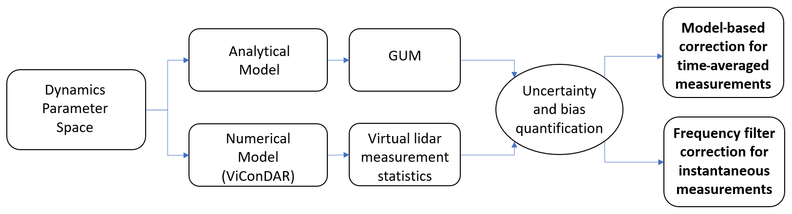
The methodology covers the introduction of the numerical and analytical models for quantification of uncertainty and bias in lidar wind measurements on floating wind turbines. A parametric study is used for the quantification of motion-induced effects. Based on the findings of the parametric study, two approaches for the correction of time-averaged and instantaneous lidar wind measurements are introduced. An overview of the methodology used and use of the analytical and numerical lidar measurement models is shown in Fig. 1. A dynamics parameter space defines the range of rotational and translational displacements. The uncertainties and biases in nacelle-based lidar measurements are quantified using the analytical model in combination with the GUM methodology and the numerical model in combination with statistical metrics. Using this quantification of uncertainties and biases, two correction approaches are introduced.

2.1 Measurement campaign

The data set analyzed for this study contains data from a forward-looking lidar mounted on the nacelle of the FLOATGEN (BWIdeol, 2019) floating wind turbine demonstrator The measurement campaign took place from December 2020 to April 2021. For this study measurement data from January 2021 were analyzed.

The floating substructure is a barge-type floater employing BW Ideol's damping pool design. It is installed on the SEM-REV test site (ECN, 2017) located near the Atlantic coast of Brittany. The wind turbine employed for this demonstrator is a 2 MW Vestas V80 turbine with a rotor diameter of 90 m and a hub height of 60 m. Further details on the measurement campaign can be found in Özinan et al. (2022).

The measurement campaign employed a Wind Iris TC lidar (Vaisala, 2022). This lidar system is a four-beam pulsed lidar with a 1 Hz sampling frequency for the total pattern. LOS velocities are measured at 10 distances from 50 to 200 m. The beam geometry of the system is described in Sect. 3.2. Furthermore, the lidar system is equipped with an IMU, providing the rotational displacement in pitch and roll direction of the lidar system. The wind field reconstruction procedure followed in this study is based on the approach from Schlipf et al. (2020). In this method the horizontal wind speed components u and v are reconstructed using LOS measurements from all four beams. For the rotational displacement measurements from the lidar IMU, it has been found that the measurements do heavily overestimate the amplitudes of the displacements compared with other nacelle-based sensors. Therefore, the inclination data used in this study have been corrected using a linear relationship between the inclination measurements of the IMU and other nacelle-mounted inclinometers. The correction approach is discussed in Chen et al. (2022).

2.2 Analytical model

The analytical uncertainty model aims to provide estimates of uncertainty for lidar LOS wind speed measurements and wind field characteristics reconstructed from LOS wind speed measurements. The uncertainty estimation according to the GUM methodology requires an analytical description of the measurement. For the case of nacelle-based lidar measurements on a FOWT, the model must contain the relevant dynamic behavior of the FOWT, a description of the wind field, and a model of the measurement itself.

Figure 2 Lidar pattern and coordinate systems for the analytical model.

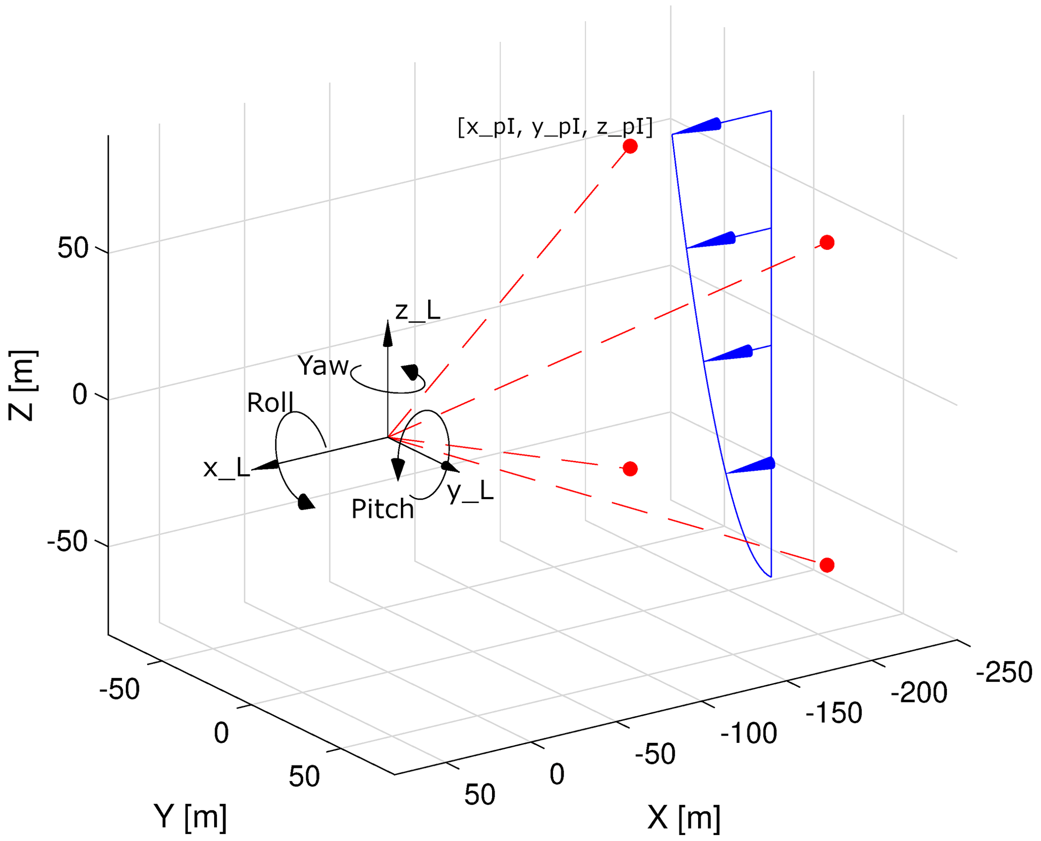
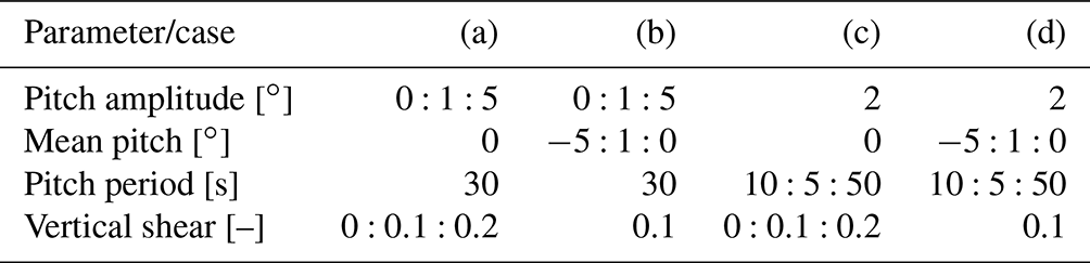
The dynamic behavior of the FOWT is modeled considering four DOFs, namely the rotational displacement in yaw, pitch, and roll direction, as well the heave displacement of the floater (see Fig. 2). The low-frequency displacements of the floater in the surge and sway direction are typically causing slow translational displacements of the nacelle compared to the effect of rotational floater displacements. Therefore, the sway and surge displacement of the floater is not considered in the model as individual DOFs. The temporal behavior of the considered DOFs, a, is modeled by harmonic oscillations around a defined mean value:

$$\begin{array}{}\text{(1)}& a=A_a\cdot \left(\sin {\displaystyle \frac{\mathrm{2}\mathit{\pi }}{T_a}}t\right)+k_a,\end{array}$$

where A_a is the amplitude, T_a is the period, k_a is the mean value of the respective DOF, and t is the time. A rigid floater-tower assembly is assumed to transfer the modeled floater dynamics to the dynamics of the lidar device mounted on the nacelle of the turbine. Therefore, the rotational displacement and the translational heave displacement of the lidar device are equivalent to the displacement of the floater. The rotational displacements of the floater cause relevant translational displacements at the mounting position of the lidar. The translational displacements $(x_{\text{trans}},y_{\text{trans}},z_{\text{trans}})$ are modeled by defining the mounting position of the lidar, $[x_{\mathrm{m}},y_{\mathrm{m}},z_{\mathrm{m}}]$, in the floater coordinate system and the multiplication by a rotation matrix R:

$$\begin{array}{}\text{(2)}& {\displaystyle }\left[\begin{array}{c}{x}_{\text{trans}}\\ y_{\text{trans}}\\ z_{\text{trans}}\end{array}\right]=\mathbf{R}(\mathit{\psi },\mathit{\beta },\mathit{\gamma })\cdot \left[\begin{array}{c}{x}_{\mathrm{m}}\\ y_{\mathrm{m}}\\ z_{\mathrm{m}}\end{array}\right]+\left[\begin{array}{c}\mathrm{0}\\ \mathrm{0}\\ z_{\text{heave}}\end{array}\right],\end{array}$$

where z_heave is the heave elevation of the floater (see Fig. 2). The definition of the rotation matrix R is given in Appendix A5. The translational velocities at the lidar mounting position are found by calculation of the first time derivative of the translational displacement:

$$\begin{array}{}\text{(3)}& {\mathit{x}}_{\text{vel}}={\displaystyle \frac{\mathrm{\Delta }{\mathit{x}}_{\text{trans}}}{\mathrm{\Delta }t}},\end{array}$$

where x_trans denotes the vector of translational displacements $(x_{\text{trans}},y_{\text{trans}},z_{\text{trans}})$, and x_vel is the vector of translational velocities $(x_{\text{vel}},y_{\text{vel}},z_{\text{vel}})$.

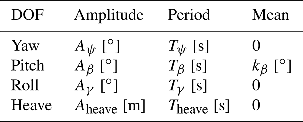
The model parameters defining the dynamic behavior of the FOWT are summarized in Table 1.

Table 1 Considered FOWT dynamics parameters.

In reality, the LOS measurement of a lidar is influenced by various atmospheric and technical parameters. For the analytical calculation of motion-induced uncertainties, a simplified model of the atmosphere and the lidar measurement is introduced. The horizontal wind speed is modeled using a power-law profile given by

$$\begin{array}{}\text{(4)}& V_{\mathrm{h}}=V_{\text{ref}}{\left({\displaystyle \frac{H}{H_{\text{ref}}}}\right)}^{\mathit{\alpha }},\end{array}$$

where V_ref is the reference wind speed, H_ref is the reference height, H is the height above ground, and α is the vertical wind shear exponent. Horizontally, the wind field is assumed to be homogeneous. The v and w wind speed components are assumed to be zero. While these assumptions avoid the introduction of a turbulence model and enable the analytical derivation of uncertainty following the GUM methodology, it should be pointed out that model results do not reflect any effects originating from the turbulent nature of real wind fields.

For the consideration of the dynamic LOS position due to floater motion, two coordinate systems are introduced. Following the notation of Schlipf (2016), the I coordinate system is an earth-fixed reference coordinate system, and the L coordinate system is the coordinate system of the lidar device. The coordinates of the lidar focus points are defined in terms of angles from the center line θ and angles around the center line ϕ:

$$\begin{array}{}\text{(5)}& {\displaystyle }\left[\begin{array}{c}{x}_{\mathrm{p},\mathrm{L}}\\ y_{\mathrm{p},\mathrm{L}}\\ z_{\mathrm{p},\mathrm{L}}\end{array}\right]=\left[\begin{array}{c}\cos \mathit{\theta }\\ \sin \mathit{\theta }\cos \mathit{\varphi }\\ \cos \mathit{\theta }\sin \mathit{\varphi }\end{array}\right].\end{array}$$

The specific beam geometry used in this study is given in Sect. 3.2. Considering the rotational displacement of the lidar system due to the yaw, pitch, and roll DOFs of the floater, the coordinates of the rotated focus points in the earth-fixed coordinate system are obtained by multiplication by a rotation matrix R:

$$\begin{array}{}\text{(6)}& {\displaystyle }\left[\begin{array}{c}{x}_{\mathrm{p},\mathrm{I}}\\ y_{\mathrm{p},\mathrm{I}}\\ z_{\mathrm{p},\mathrm{I}}\end{array}\right]=\mathbf{R}(\mathit{\psi },\mathit{\beta },\mathit{\gamma })\cdot \left[\begin{array}{c}{x}_{\mathrm{p},\mathrm{L}}\\ y_{\mathrm{p},\mathrm{L}}\\ z_{\mathrm{p},\mathrm{L}}\end{array}\right].\end{array}$$

where $\mathit{\psi },\mathit{\beta },$ and γ are the current roll, pitch, and yaw angle, respectively, and $(x_{\mathrm{p},\mathrm{I}},y_{\mathrm{p},\mathrm{I}},z_{\mathrm{p},\mathrm{I}})$ is the current position of the lidar focus points in earth-fixed coordinates (see Fig. 2). The rotation matrix R is given in Appendix A5.

Finally, the LOS velocity is mathematically described by a projection of the local wind vector $[u,v,w]$ on the vector describing the line of sight. In the remainder of the paper, we refer to u as the u component of the wind field.

$$\begin{array}{}\text{(7)}& {\mathit{v}}_{\text{los}}=x_{\text{pn},\mathrm{I}}u+y_{\text{pn},\mathrm{I}}v+z_{\text{pn},\mathrm{I}}w+(x_{\text{In}}{x}_{\text{vel}}+y_{\text{pn},\mathrm{I}}{y}_{\text{vel}}+y_{\text{pn}},z_{\text{vel}}),\end{array}$$

where $x_{\text{pn},\mathrm{I}},y_{\text{pn},\mathrm{I}},z_{\text{pn},\mathrm{I}}$ is the normalized LOS vector. The wind speed components $u,v,w$ are derived using Eq. (4). To enable a straightforward analytical uncertainty derivation, probe volume averaging effects are not considered. The translational velocities $(x_{\text{vel}},y_{\text{vel}},z_{\text{vel}})$ are added to the local wind vector as additional velocity components.

The dynamic measurement height H is given by

$$\begin{array}{}\text{(8)}& H=z_{\mathrm{p},\mathrm{I}}+h_{\text{lidar}}+h_{\text{heave}},\end{array}$$

where z_p,I is the z coordinate of the focus point, h_lidar is the height of the lidar mounting position above mean sea level, and h_heave is the elevation due to the heave motion of the floating platform.

Considering the vertical wind profile and the wind direction φ and assuming the vertical wind speed component w to be zero yields

$$\begin{array}{}\text{(9)}& \begin{array}{rl}{v}_{\text{los}}& =V_{\text{ref}}{\left({\displaystyle \frac{z_{\mathrm{p},\mathrm{I}}+h_{\text{lidar}}+h_{\text{heave}}}{H_{\text{ref}}}}\right)}^{\mathit{\alpha }}\\ & \times (\sin \mathit{\phi }\cdot x_{\text{pn},\mathrm{I}}+\cos \mathit{\phi }\cdot y_{\text{pn},\mathrm{I}})\\ & +(x_{\text{pn},\mathrm{I}}{x}_{\text{vel}}+y_{\text{pn},\mathrm{I}}{y}_{\text{vel}}+y_{\text{pn},\mathrm{I}}{z}_{\text{vel}}).\end{array}\end{array}$$

Following the recommendation of IEC 61400-50-3:2022 (2022), the GUM methodology is applied for quantification of uncertainty in v_los as a function of input parameters given in Eq. (9). Further, this uncertainty is propagated through a wind field reconstruction algorithm to derive uncertainties of the reconstructed u component of the wind vector. Details on the derivation of uncertainty are described in Appendix A. The analytical model is also used to quantify the bias in lidar-estimated u-component wind speed as a function of dynamic input parameters. The derivation of bias is given in Appendix A3. The model is made available as an open-source tool by the chair for wind energy at the University of Stuttgart (SWE) on https://github.com/SWE-UniStuttgart/FLIDU (last access: 27 April 2023).

2.3 Numerical model

The analytical model for the estimation of uncertainty and biases introduced in Sect. 2.2 includes several simplifying assumptions about the wind field and the measurement. Particularly, it assumes a horizontally homogeneous wind field, does not account for turbulent effects, and models the lidar measurement as a single-point measurement. Therefore, a more sophisticated numerical model is employed to verify the analytical uncertainty and bias estimation. ViConDAR is an open-source numerical framework for the simulation of lidar measurements in turbulent wind fields and the use of simulated measurements as constraints in synthetic wind field generation. Details on ViConDAR can be found in Pettas et al. (2020). ViConDAR has been adapted for consideration of floating dynamics of the lidar system in six DOFs. In this study, we use ViConDAR to simulate lidar measurements under the same dynamic input quantities as in the analytical model and derive uncertainties and biases of simulated measurements and reconstructed wind speed. ViConDAR requires the input of the rotational displacements (yaw, pitch, roll); the translational displacements in surge, sway, and heave direction; and the translational velocities in the surge, sway, and heave direction.

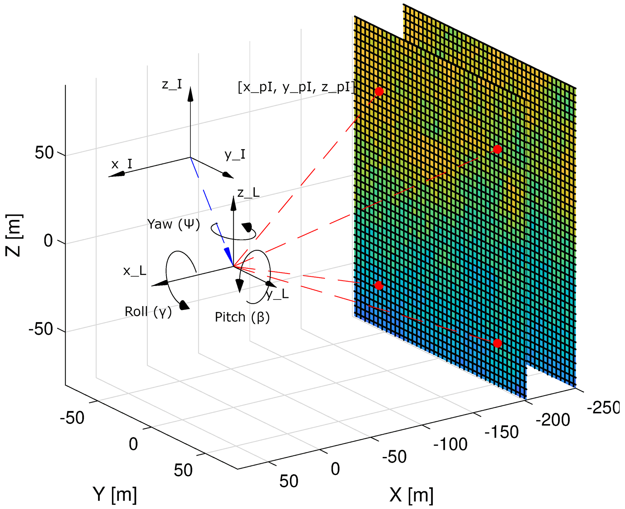
Similar to the analytical model, the positions of lidar focus points after rotational displacement are obtained by multiplication of the LOS vectors by a rotation matrix $R(\mathit{\psi },\mathit{\beta },\mathit{\gamma })$. The translational displacement of the lidar system does not affect the angular beam directions but shifts the lidar system and the focus in space. After consideration of translational displacements the positions of focus points are given by

$$\begin{array}{}\text{(10)}& {\displaystyle }\left[\begin{array}{c}{x}_{\mathrm{p},\mathrm{I}}\\ y_{\mathrm{p},\mathrm{I}}\\ z_{\mathrm{p},\mathrm{I}}\end{array}\right]=\mathbf{R}(\mathit{\psi },\mathit{\beta },\mathit{\gamma })\cdot \left[\begin{array}{c}{x}_{\mathrm{p},\mathrm{L}}\\ y_{\mathrm{p},\mathrm{L}}\\ z_{\mathrm{p},\mathrm{L}}\end{array}\right]+\left[\begin{array}{c}{x}_{\text{trans}}\\ y_{\text{trans}}\\ z_{\text{trans}}\end{array}\right],\end{array}$$

where $(x_{\mathrm{p},\mathrm{L}},y_{\mathrm{p},\mathrm{L}},z_{\mathrm{p},\mathrm{L}})$ is the focus point position in lidar coordinates, ($x_{\text{trans}},y_{\text{trans}},z_{\text{trans}}$) are the translational displacements and include the surge, sway, and heave DOFs of the floating platform.

The LOS measurements of the individual beams are modeled as a projection of the wind vector $[u,v,w]$ on the current normalized LOS vector $(x_{\text{pn},\mathrm{I}},y_{\text{pn},\mathrm{I}},z_{\text{pn},\mathrm{I}})$:

$$\begin{array}{}\text{(11)}& \begin{array}{rl}{v}_{\text{los}}& =\underset{-\mathrm{\infty }}{\overset{\mathrm{\infty }}{\int }}(x_{\text{pn},\mathrm{I}}u+y_{\text{pn},\mathrm{I}}v+z_{\text{pn},\mathrm{I}}w)f\left(a_{\mathrm{d}}\right)d{a}_{\mathrm{d}}\\ & +(x_{\text{vel}}{x}_{\text{pn},\mathrm{I}}+y_{\text{vel}}{y}_{\text{pn},\mathrm{I}}+z_{\text{vel}}{z}_{\text{pn},\mathrm{I}}),\end{array}\end{array}$$

where f(a_d) is the range-weighting function, and a_d is the distance between the lidar and the focus point. In the simulation, the range-weighting function is represented by a definable length of the range gate and discretized by a number of points along the beam. The length of the range gate is set to 30 m, discretized over 10 points. The translational velocities $(x_{\text{vel}},y_{\text{vel}},z_{\text{vel}})$ of the lidar create additional velocity components in the LOS measurements. The x coordinate of the focus points in space is converted to the time coordinate of the synthetic turbulence box using Taylor's frozen turbulence hypothesis. The wind vector is then sampled from the closest point to the $[x,y,z]$ grid of the synthetic turbulence box (see Fig. 3).

Figure 3 Lidar pattern and coordinate systems for the numerical model.

Synthetic turbulent wind fields with desired characteristics are created using a turbulence generator. In this work the open-source turbulence generator TurbSim (Jonkman, 2014), which is based on employing the Veers method (Veers, 1988) for turbulence modeling, is used. The u-component wind speed is reconstructed following the same approach as the reconstruction procedure for the analytical model described in Appendix A2.

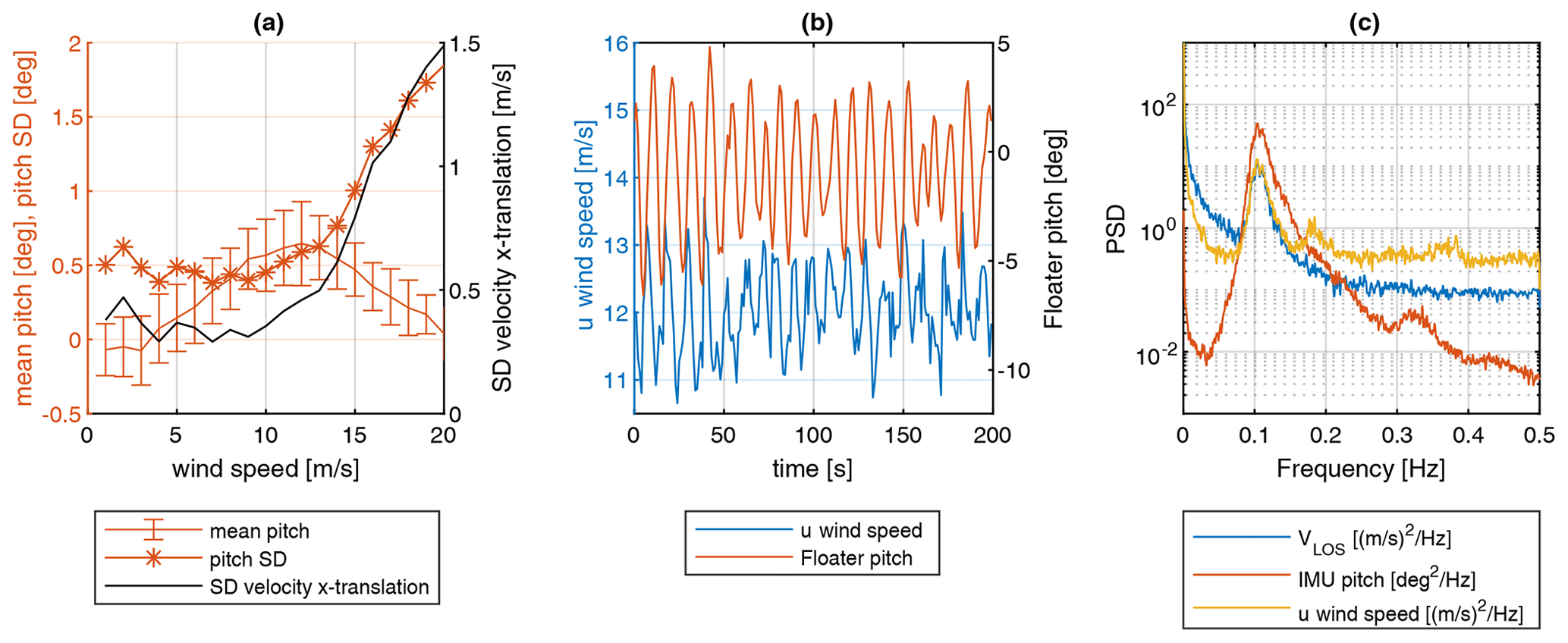
Figure 4 Analysis of measurement campaign data. (a) Mean and standard deviation of floater pitch angle over 10 min mean wind speed bins. Error bars denoting the standard deviation of mean pitch values over all 10 min samples. Standard deviation of translational velocity in x direction over wind speed bins. (b) Time series of reconstructed u-component wind speed and pitch angle. (c) PSD of floater pitch angle, LOS-1 velocity, and reconstructed u-component wind speed.

3 Motion influence in nacelle-based lidar measurements

3.1 Findings from measurement campaign

Figure 4a shows the 10 min inclination sensor mean pitch angle per wind speed, including the standard deviation of the 10 min mean pitch angle per wind speed bin for the floating example data set. As expected the mean pitch angle data show a high dependency on wind speed and related thrust force. However, the magnitude of mean pitch angles is in the region below 1^∘, which is rather low compared to other floater types (e.g., Windcrete FOWT concept; Mahfouz et al., 2021).

Additionally, the standard deviation within each 10 min interval is shown per wind speed bin. Standard deviations in the pitch angle are increasing with the wind speed and the associated wave excitation of the floater. For this floater type, the pitch motion is mainly caused by hydrodynamic forces and is large compared to other floater types (e.g., spar-type floaters). This pitch motion causes translational velocities of the nacelle in the x direction. In Fig. 4a, the black line shows the standard deviation of the translational velocity in the x direction.

Since this velocity component is superimposed on the measurement, it can be expected that the pitch motion and related translational velocities of the nacelle will cause significant fluctuations in the lidar measurements. The effect of mean pitch angles and related shift of measurement positions is expected to have a smaller influence on the measurement for this floater type.

This is confirmed by the time series example in Fig. 4b, which shows the lidar-reconstructed wind speed estimate and the measured pitch inclination signal. A strong correlation between the pitch angle of the floater and the lidar wind speed can be observed.

Finally, the power spectral density (PSD) of the inclination pitch signal and one LOS velocity signal as well as the reconstructed u component of the wind speed are shown in Fig. 4c. The PSDs of the LOS velocities of the individual beams and the pitch signal and the reconstructed u component of the wind speed show peaks at the floater pitch frequency. For this example, a clear correlation between the lidar pitch signal and the reconstructed u-component wind speed can be observed. This analysis shows that the rotational DOF of the floater, in particular the pitch motion, is strongly influencing the LOS measurements and the reconstructed wind speed of the nacelle-mounted lidar. These findings suggest that the motion influence on the lidar measurements needs to be further investigated and quantified.

3.2 Parametric study for uncertainty and bias quantification

In this section the findings from uncertainty and bias estimation of lidar measurements under motion influence, as defined in Appendix A, are presented for both the analytical and the numerical approach. The lidar configuration investigated in the numerical and analytical uncertainty estimation follows the one which is used in the real measurement campaign.

This configuration represents a fixed-beam lidar system with four beams, arranged in a rectangular pattern. The opening angle (angle to the center line) of all four beams is set to θ = 19.8^∘, and the angle around the center line is set to ϕ = 39.6, 140.4, −39.6, and −140.4^∘. The range of the lidar is assumed to be 200 m. The LOS measurements from all four beams are taken sequentially with a delay of T_meas = 0.25 s. For this pattern, the duration of a full scan is 1 s. The resulting scanning pattern is visualized in Fig. 3. For both the analytical model and the numerical model, a hub height, which is also the installation height of the lidar, of 100 m and a rotor radius of 75 m are assumed.

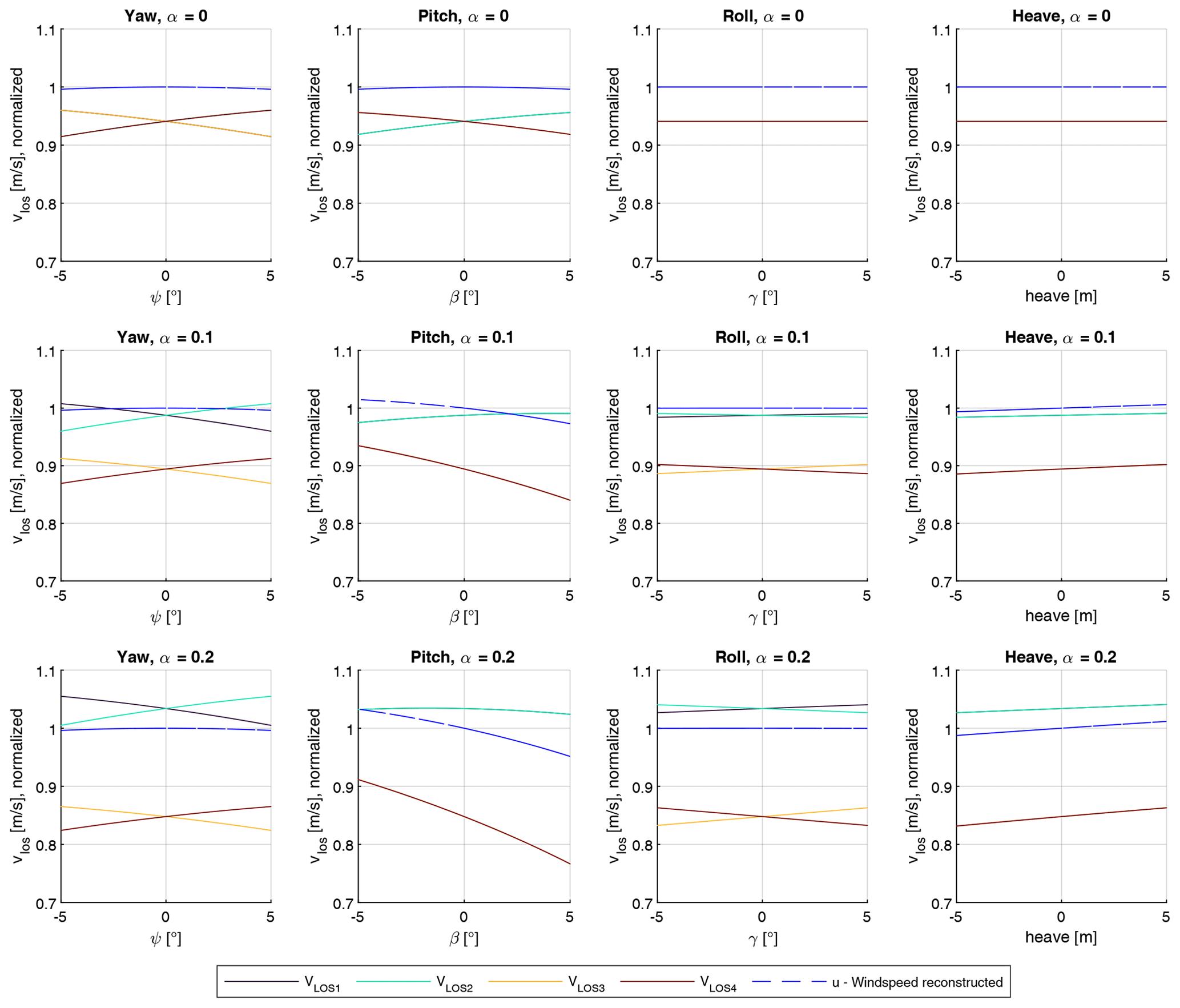
Figure 5 Modeled LOS velocities and reconstructed u-component wind speed as a function of yaw, pitch, roll, and heave displacement for all four beams. Reference wind speed: 10 m s⁻¹. Top: α=0. Center: α=0.1: Bottom: α=0.2. α is the vertical shear exponent. V_LOS1 and V_LOS2 correspond to the two upper beams, and V_LOS3 and V_LOS4 correspond to the two lower beams. The y axis is normalized to the reconstructed wind speed at zero displacements.

In the first analysis, the influence of displacement in individual DOFs on the measured LOS velocities is examined with the help of the analytical model. Figure 5 shows the LOS velocity per beam as a function of displacement for the yaw, pitch, roll, and heave displacement for three values of the vertical shear exponent α. Additionally, the reconstructed u component of the wind field is shown as a function of each DOF. The reconstruction approach is detailed in Appendix A2. In this analysis, quasi-static displacements are assumed. Velocity components resulting from changing quasi-static conditions are not considered.

For a vertical shear exponent of α=0, the individual LOS velocities differ for changing pitch and yaw angles. However, due to the symmetric beam pattern, the reconstructed wind speed shows no significant fluctuation over the respective DOF. Under the presence of a vertical wind shear profile, this behavior changes. The yaw and roll displacement causes fluctuations in the LOS velocities. Again the reconstructed wind speed stays nearly constant due to the symmetric beam pattern.

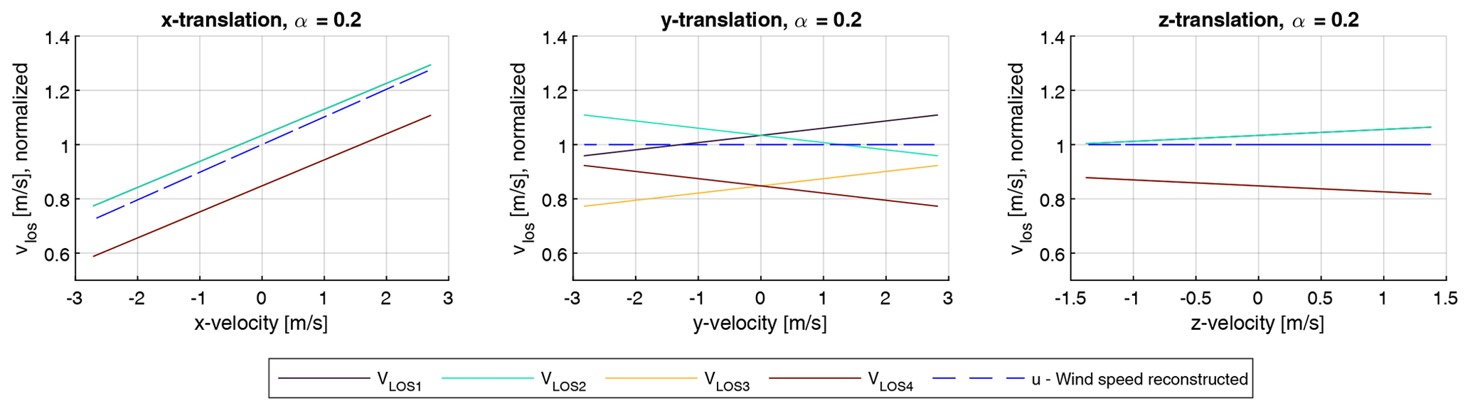
Figure 6 Modeled LOS velocities as a function of translational nacelle velocities in x, y, and z directions for all four beams. Reference wind speed: 10 m s⁻¹ and vertical shear exponent α=0.2. The y axis is normalized to the reconstructed wind speed at zero displacements.

For the pitch DOF, the upper and lower beam LOS velocities have different characteristics. Therefore, the reconstructed wind speed is fluctuating. It is also important to note that the relationship between reconstructed wind speed and pitch angle is nonlinear. This nonlinear relationship can cause bias in averaged lidar wind speed estimates. Heave displacement in combination with a nonlinear vertical wind shear profile causes fluctuation in the reconstructed wind speed due to changing measurement elevation. As a result, the reconstructed u-component wind speed will show a small negative bias because horizontal wind speeds increase slower with increasing height than they decrease with decreasing height. However, for the expected range of floater heave elevations, this effect is small compared to the effect of floater pitch motion.

Figure 6 illustrates the dependency of measured LOS velocities and reconstructed wind speed on translational velocities of the lidar device for quasi-static conditions. No fluctuation in translational velocities is considered. It can be seen that the translational velocity components are directly projected on the LOS direction of the beam and thus cause significant changes in the measured LOS velocities. For the translational displacement in the x direction, this directly translates into changing reconstructed wind speeds. For the y and z direction the reconstructed u-component wind speed remains constant, since the effects on the left and right as well as upper and lower beams compensate for each other. However, it is important to note that the relationship is strictly linear, meaning that zero mean fluctuations in translational velocities will cause zero mean fluctuations in LOS velocities and thus not cause any bias in the LOS velocity and reconstructed u component of the wind speed.

This analysis shows that the most relevant DOF for the influence of nacelle-based lidar wind measurements is pitch motion. Under the presence of a vertical wind shear profile, the rotational pitch displacement causes a significant variation in reconstructed wind speed. This variation is nonlinear as a function of pitch displacement, indicating that the displacement could introduce bias in the measurement. The rotational pitch motion also causes translational velocities of the nacelle in the x direction. These translational velocities cause fluctuations in the reconstructed wind speed. Consequently, we focus on the analysis of the influence of the pitch DOF in combination with the present vertical shear profile in the following sections.

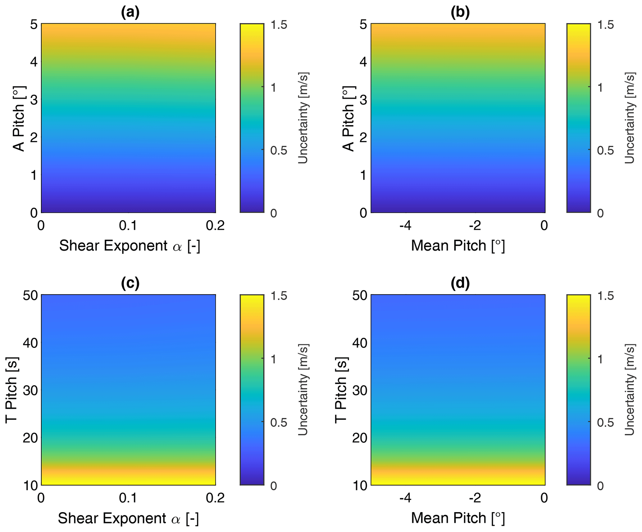
Figure 7 Uncertainty estimation of u-component wind speed. Fixed parameters: U_ref = 10 m s⁻¹, A_ψ = 0^∘, A_γ = 0^∘, and A_heave = 0m.

3.3 Uncertainty quantification

In this section, we quantify motion-induced uncertainties in reconstructed lidar wind speed estimates as a function of dynamic input parameters using the analytical and numerical models. For the analytical model, the wind field is only defined by the inflow wind speed of 10 m s⁻¹ and the vertical shear exponent α. The dynamics parameters are summarized in Table 2. Figure 7a and b show the u-component wind speed uncertainty estimates from the analytical model as functions of shear exponent, mean pitch angle, and pitch amplitude.

Table 2 Dynamics parameters for uncertainty quantification.

The resulting uncertainty of the reconstructed u wind speed component is mainly dependent on the pitch amplitude, which determines the magnitude of different effects. With a given pitch period of 30 s, the pitch amplitude determines the magnitude of the translational velocity in the fore–aft direction. In this case, this is the main source of uncertainty in the reconstructed wind speed. Additionally, the pitch amplitude determines the uncertainty resulting from changed beam direction and shifted focus points. The overall uncertainty of the u wind speed component is found to be in the region of up to 315 % of the reference wind speed. No significant influence of the inflow shear exponent and the mean pitch angle on the overall uncertainty estimate of the u-component wind speed component can be observed.

In the next step, the influence of the frequency of rotational pitch movement was investigated. Figure 7c and d show the uncertainty of u-component wind speed as a function of shear exponent, mean pitch angle, and period of floater pitch movement. The corresponding parameter space is summarized in Table 2. Results show a strong dependency on the period of the rotational pitch movement of the floater. This parameter determines the magnitude of the translational velocities at the lidar mounting position. Therefore, short periods of rotational movement in general cause high uncertainty in u-component wind estimates. No significant influence of the inflow shear exponent and the floater mean pitch angle can be observed.

Verification of the analytical results is done employing the numerical model. Turbulent synthetic wind fields used in the simulations are generated for a mean wind speed of 10 m s⁻¹ and a turbulence intensity of 6 %. A total of 10 random turbulence realizations are generated for each wind condition, and the presented results are averaged over all random realizations. Additional wind field parameters are summarized in Table 3.

Table 3 Wind field parameters.

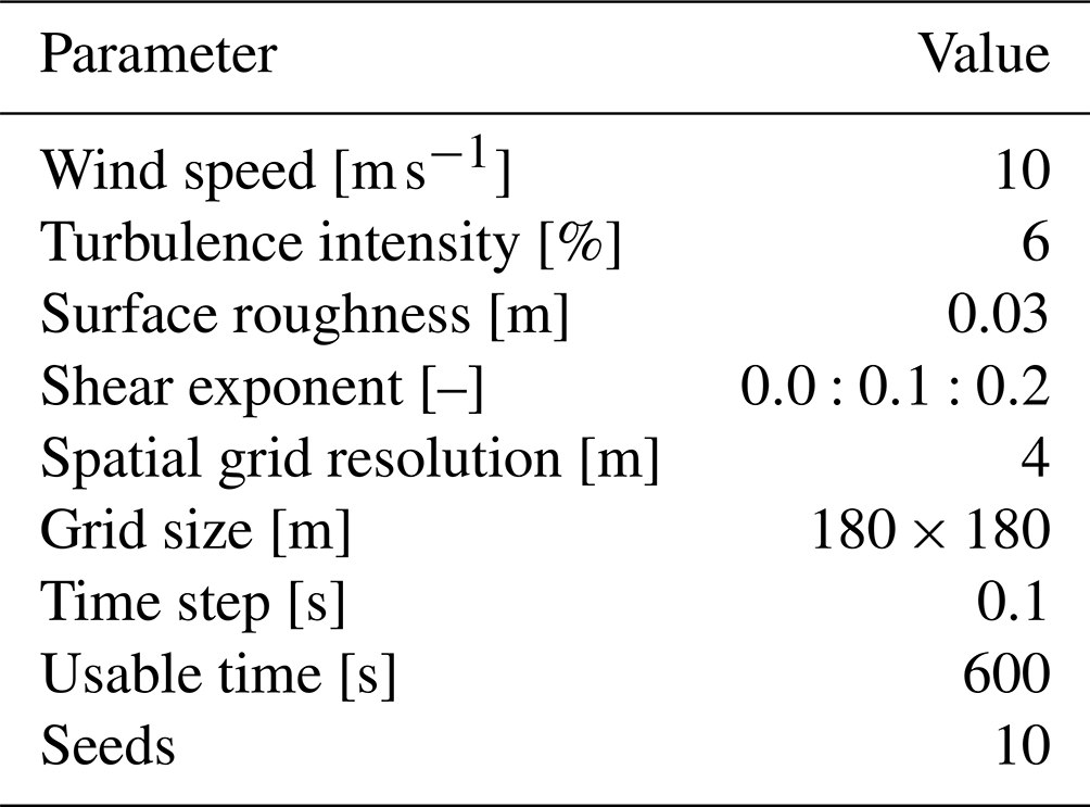
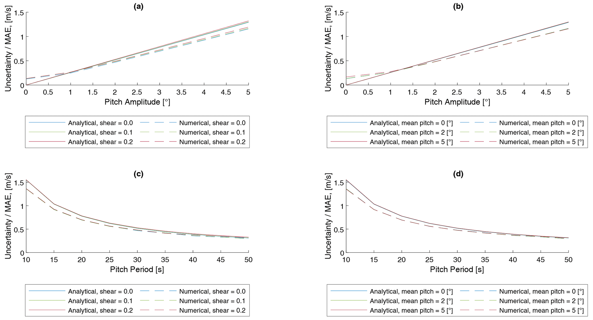
Figure 8 Comparison between analytical and numerical uncertainty and MAE estimation. Panels (a) to (d) refer to cases in Table 2. Fixed parameters: U_ref = 10 m s⁻¹, A_ψ = 0^∘, A_γ = 0^∘, and A_heave = 0 m.

Figure 8 shows a comparison of the analytical and numerical uncertainty estimation for selected dynamic input parameters. For the numerical model, uncertainty is represented by the mean absolute error (MAE) metric. The MAE is the mean of the absolute error between the time series of lidar-estimated wind speed and the reference time series of the full input wind field. The MAE represents the instantaneous error between the reconstructed wind speed and the input wind field. Therefore, it contains the fluctuations resulting from assumed FOWT dynamics. This metric can be compared qualitatively and quantitatively to the uncertainty results from the analytical model.

In general, the pattern of the numerical results follows the estimation of the analytical uncertainty model. The MAE is heavily dependent on the pitch amplitude and period, which is determining the magnitude of the fore–aft motion of the lidar system. The shear exponent and mean pitch angle variation show no significant effect on the MAE. Quantitatively, both models show similar magnitudes of uncertainty and MAE values. It can be seen that there is a linear relationship between uncertainty in the u-component wind speed estimate and the amplitude of the pitch DOF of the floater. A nonlinear relationship between uncertainty in u wind speed estimate and pitch period with lower uncertainties for increasing pitch periods can be observed.

This analysis shows that the uncertainty in reconstructed u-component wind speed measurements is dominantly determined by the fore–aft motion of the nacelle, which is mainly caused by the pitch rotation of the floater. High pitch amplitudes and high frequencies cause high uncertainties in wind speed estimates. For the conditions and models considered, this uncertainty is found to be of the order of magnitude of 1 m s⁻¹.

3.4 Bias quantification

In this section, we quantify the motion-induced bias in reconstructed lidar wind speed estimates as a function of dynamic input parameters using the analytical and numerical models. The input wind fields for the numerical model and the dynamics parameter space are the same as previously used for the uncertainty quantification.

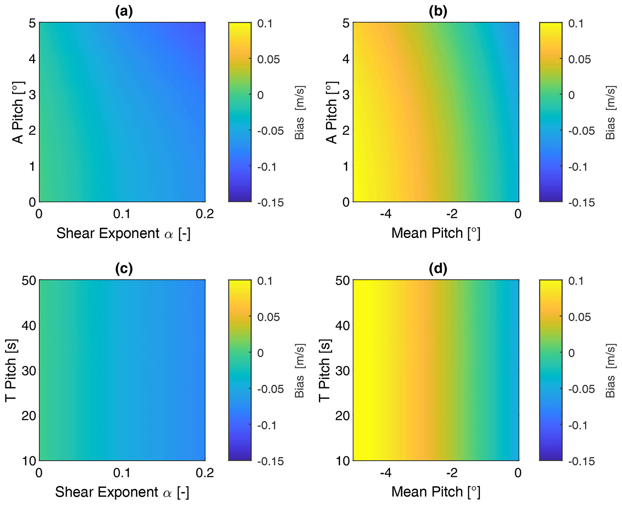
Figure 9 Bias of u-component wind speed. Parameter according to Table 2. Fixed parameters: U_ref = 10 m s⁻¹, A_ψ = 0^∘, A_γ = 0^∘, and A_heave = 0 m.

Figure 9a and b show the estimation of bias in the reconstructed u-component wind speed from the analytical model. As a function of vertical shear exponent and pitch amplitude, results show a negative bias in the reconstructed u-component wind speed, which is increasing for higher shear exponents. For increasing pitch amplitudes a slightly negative trend in the wind speed estimation can be observed, which is more pronounced for high vertical shear conditions. This is caused by the combined effect of a nonlinear vertical wind shear profile and the nonlinear relationship between beam directions and measured LOS velocity.

Non-zero mean pitch angles result, in general, in upwards- or downwards-shifted focus points. For negative mean pitch angles (upwards-shifted focus points) and the assumption of a power-law wind profile, this results in a positive bias in the LOS measurements. Depending on the magnitude of vertical shear this effect exceeds the negative effect from the pitch motion and leads to an overestimation of wind speed. Consequently, the overestimation is most pronounced for high negative mean pitch and low pitch amplitudes.

For the relationship between vertical shear, pitch amplitude, and resulting bias, it can be seen that the calculated bias is not 0, even in the presence of zero pitch amplitude. This bias is not introduced by any dynamics but is a result of the definition of the reference value used for bias calculation. As detailed in Appendix A, the reference for bias calculation is defined as the average wind speed over the rotor plane. Depending on the present shear profile, the assumed rotor size, and the lidar pattern, this reference value is different from the lidar u-component wind speed estimate. Therefore, only the change of bias over the varying dynamics parameters can be attributed to the influence of the dynamics.

Figure 9c and d show the bias of u-component wind speed as a function of shear exponent, mean pitch angle, and pitch period. No significant dependency of wind speed bias to the frequency of the floater pitch motion can be observed.

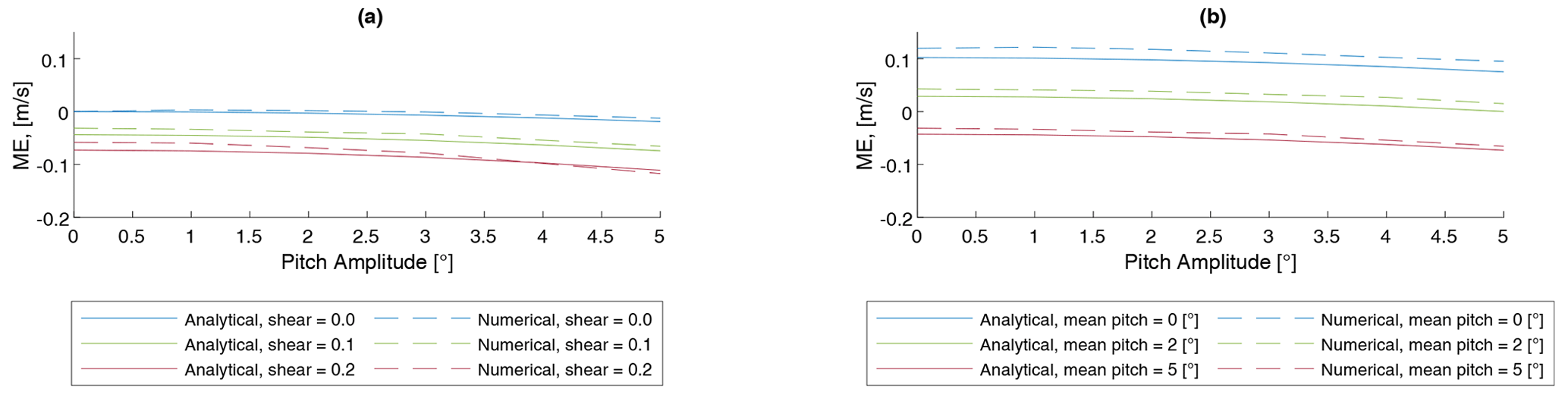
Figure 10 Comparison of bias wind speed estimation from the analytical and numerical model. Fixed parameters: U_ref = 10 m s⁻¹, A_ψ = 0^∘, A_γ = 0^∘, A_heave = 0 m, and α=0.1.

The analytical model results are verified using the numerical model. Figure 10 shows a comparison between the numerical and analytical bias estimation. For the numerical model, the bias is expressed in terms of the mean error (ME), which is the error between the mean of the lidar-estimated time series and the mean of the full wind field time series over the full simulation length of 600 s. The ME can be compared to the bias metric from the analytical model. As for the uncertainty estimation, the ME follows the pattern of the analytical bias estimation. Quantitatively, the results of both models show good agreement. Observed deviations between the model results are in the region below 0.015 m s⁻¹ for the given reference wind speed of 10 m s⁻¹.

This analysis shows that the bias in reconstructed u-component wind speed is determined by the mean pitch angle of the floater and the pitch amplitude. In the presence of vertical wind shear, negative mean pitch angles cause upwards-shifted focus points, which result in positive bias in u-component wind speed estimates. High pitch amplitudes cause negative bias in u-component wind speed estimates. This bias is of the order of magnitude of 0.1 m s⁻¹.

4 Correction approaches

The results of the numerical and analytical uncertainty and bias estimation have identified the main dynamic effects influencing the measurements of nacelle-based lidars on floating wind turbines. Motion-induced uncertainties in measurement time series are mainly influenced by the following:

• Translational velocity components caused by the fore–aft movement of the nacelle due to floater pitch motion cause fluctuation in horizontal wind speed estimates.

Motion-induced biases in time-averaged wind speed measurements are mainly influenced by the following:

• Rotational oscillations of the beam direction due to floater pitch motion cause an underestimation of horizontal wind speed components.

• Negative mean pitch angles of the FOWT are causing upwards-shifted focus points, resulting in an overestimation of wind speed.

It is important to note that these effects have different orders of magnitude and are relevant at different timescales. Translational velocities cause fluctuations in the measurement time series, which can be of the order of 1 m s⁻¹, and must be considered when using measurement time series data. Overestimation and underestimation of mean wind speeds due to rotational movement are 1 order of magnitude smaller and are found to be in the region of 0.1 m s⁻¹. This is most relevant in cases where accurate estimates of mean wind speed are necessary.

Depending on the intended use of the measurement, a correction of these effects can be necessary. Power performance measurement of wind turbines is a key application of lidar wind measurements. According to IEC 61400-12-1, the performance measurements should be performed by measuring the 10 min average power output of the wind turbine and the 10 min average inflow wind speed. A wind turbine power curve is then obtained by binning the wind speeds from 4 to 16 m s⁻¹ and plotting against the corresponding power outputs. While the standard procedure requires the use of met-mast-mounted cup anemometers, the use of nacelle-based lidar is an attractive alternative. However, the question arises if wind speed measurements from nacelle-mounted lidars introduce uncertainty or bias in the power performance measurements and if motion-induced effects need to be corrected. The findings from Sect. 3.4 show that mean wind speed estimates from nacelle-based lidars can be biased depending on the dynamic condition of the wind turbine. For power performance measurements, bias of the order of 0.1 m s⁻¹ or around 1 % could be significant. This suggests that a correction of 10 min mean wind speed estimates, used for power performance assessment, will be necessary for the use of nacelle-based lidar systems on floating wind turbines under specific dynamic conditions.

The use of lidar inflow measurements for turbine load validation has been investigated by several studies using different methods. In Conti et al. (2020) 10 min statistics of lidar-estimated wind field characteristics are used for the parameterization of synthetic turbulent wind fields for aeroelastic turbine simulations and evaluation of loads. It was found that uncertainties in the lidar-estimated mean wind speed and the lidar-estimated turbulence intensity used for the parameterization of synthetic wind fields are the main sources of uncertainty in predicted loads. It can be expected that the dynamics-induced bias in lidar wind speed measurements will affect load estimations. In Dimitrov et al. (2019), besides lidar-estimated wind field statistics for parameterization, measured lidar wind speed time series are used to constrain synthetic wind fields for load validation studies. In this method, it can be expected that motion-induced fluctuations in the wind speed measurements will significantly influence the resulting wind field and load estimates. This suggests that the correction of instantaneous errors in lidar wind speed measurements is necessary for use in load validation studies.

Another application of nacelle-based lidar systems on FOWT is the use of lidar wind speed measurements for turbine pitch control. Here the wind speed information of the inflow wind field is used as an input to an additional control loop that aims to compensate for changes in wind speed, e.g., through gusts, by changing the rotor blade pitch angles in order to maintain the rotor speed. This control approach can significantly reduce platform motions and variations in rotor speed due to disturbance in the form of wind gusts (see, e.g., Schlipf et al., 2015). The application relies on instantaneous time series information of the inflow wind speed with sampling frequencies in the region of 1 Hz. Since these measurements contain motion-induced fluctuations, correction of the lidar wind speed measurement time series data is necessary to avoid undesired effects on the pitch controller. In Schlipf et al. (2015) this is considered by using a model-based wind field reconstruction algorithm, which takes the instantaneous displacements and velocities of the lidar system into account, to provide a motion-compensated wind speed estimate.

The abovementioned use cases show that motion correction of measurements from nacelle-based lidar systems is necessary, while different timescales have to be considered. In this work, we suggest a method for the correction of fore–aft motion-induced fluctuation based on frequency filtering and a simple model-based correction approach of the turbine mean pitch employing the analytical model.

4.1 Model-based correction

As shown in Sect. 3, the bias in the wind speed estimation is mainly caused by a non-zero mean pitch angle, which causes upwards-shifted measurement positions and oscillating beam directions, caused by the floater pitch motion.

Instead of correcting lidar measurement time series based on the instantaneous turbine tilt angles, we suggest correcting the reconstructed wind speed with a model-based approach. The analytical model introduced in Sect. 2.2 is used to calculate the mean error in the reconstructed u-component wind speed estimation as a function of the wind speed WS, vertical shear exponent α, turbine mean pitch β_mean, and pitch amplitude A_β.

$$\begin{array}{}\text{(12)}& v_{\text{corr.}}=f(\mathrm{WS},\mathit{\alpha },{\mathit{\beta }}_{\text{mean}},A_{\mathit{\beta }})\end{array}$$

In this way a four-dimensional look-up table with correction values v_corr. is created for the parameter space given in Table 4.

Table 4 Parameter space correction look-up table.

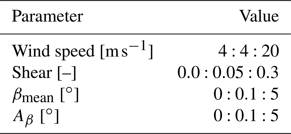
The remaining model parameters are set to fixed values of T_β = 30 s, A_ψ=0, A_γ=0, and A_heave=0, as results are only evaluated for these values. It should be mentioned that the dimension of the created correction look-up table can easily be extended to other model parameters if a significant sensitivity is found for a specific setup.

Assuming the mean pitch angle and the mean pitch amplitude are known for each 10 min period through inclination measurements and using the lidar-estimated u-component wind speed and vertical shear exponent, the correction value can be extracted from the look-up table and subtracted from the lidar-estimated u-component wind speed:

$$\begin{array}{}\text{(13)}& u_{\text{corr.}}=u_{\text{rec}}-v_{\text{corr}}(u_{\text{rec}},{\mathit{\alpha }}_{\text{rec}},{\mathit{\beta }}_{\text{mean}},A_{\mathit{\beta }}).\end{array}$$

The approach avoids the need for synchronized motion time series data, which might not be available in all cases. Inclination sensor signals might be noisy or not accurate enough due to the influence of nacelle acceleration on the sensor. Thus, the suggested approach is easy to implement for practical applications. However, it relies on the availability and accuracy of floater dynamics statistics. Inaccuracies could occur in transient conditions, where mean floater dynamics do not represent the actual floater dynamics sufficiently.

4.2 Frequency filtering

In this study, we investigate the use of frequency filters for the correction of motion-induced fluctuations. We suggest the application of a frequency filter on the time series of reconstructed u-component wind speed estimates. As shown in Fig. 4, the time series of LOS wind speed and the reconstructed u wind speed show peaks at the floater pitch frequency. The application of a frequency filter aims to correct the influence of floater pitch displacement and the resulting translational velocities in the fore–aft direction without introducing bias or error in the estimation of the real wind field properties.

For frequency filtering, we use a bandstop filter characterized by three parameters. The stopband frequency range is given by a width parameter, defining the upper- and lower-frequency limit of the stopband. The peak pitch frequency of the floater is used as the center frequency f_center of the applied bandstop filter, while the upper and lower bounds of the filter are defined at $f_{\text{pass,lower}}=f_{\text{center}}-\mathrm{width}/\mathrm{2}$ and $f_{\text{pass,upper}}=f_{\text{center}}+\mathrm{width}/\mathrm{2}$. The filtering depth is defined by the stopband attenuation parameter, depth, in dB. The steepness of the filter's transition region is defined by a steepness parameter.

The filter parameters applied in Sect. 5 are optimized with a parametric study, evaluating the ME and the MEA between the corrected lidar wind speed and the full wind field reference. The goal of this optimization is to find the filter parameterization, which is minimizing the MEA, while not increasing the ME significantly. The filter has been implemented using the MATLAB (MATLAB, 2020) bandstop filtering function.

5 Results

We evaluate the correction approaches using the numerical lidar simulation framework ViConDAR. Lidar measurements are simulated by coupling an aeroelastic simulation of specific FOWT models to ViConDAR. In this way, the dynamics input response to wind and wave conditions is used as an input to the lidar simulation. Details on the coupling approach can be found in Gräfe et al. (2022). For this study, we use two different FOWT models with different characteristics in their input response to wind and wave conditions.

The first FOWT model employed for the simulation of FOWT dynamics is the Windcrete floater design concept (Mahfouz et al., 2021) in combination with the International Energy Agency (IEA) 15 MW reference wind turbine (Gaertner et al., 2014). Windcrete is a monolithic spar design with a draft of 155 m and a tower height of 129.5 m. The hub height of this FOWT concept is 140 m above sea level. The floater and the tower are designed as a single concrete member with an overall mass of 3.665 × 10⁷ kg. Three delta-shaped catenary mooring lines are employed for station keeping of the floater. The mooring lines have an overall length of 615 m and a mass per length of 561.25 kg m⁻¹. Details on the Windcrete design parameters and the dynamic behavior can be found in Mahfouz et al. (2021). The second FOWT model is the numerical model of the FLOATGEN FOWT demonstrator, introduced in Sect. 2.1. Both FOWTs are modeled in the open-source aeroelastic simulation code OpenFAST (Jonkman, 2007). To minimize the influence of transient effects, the first 600 s of each simulation is discarded. Simulations are created for three sets of wave conditions using a JONSWAP wave spectrum with parameters given in Table 6. Turbulent synthetic wind fields are created according to parameters given in Table 5. For all testing cases the same lidar configuration as described in Sect. 3.2 is used.

Table 5 Wind field parameters.

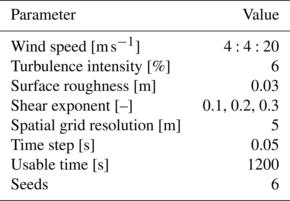
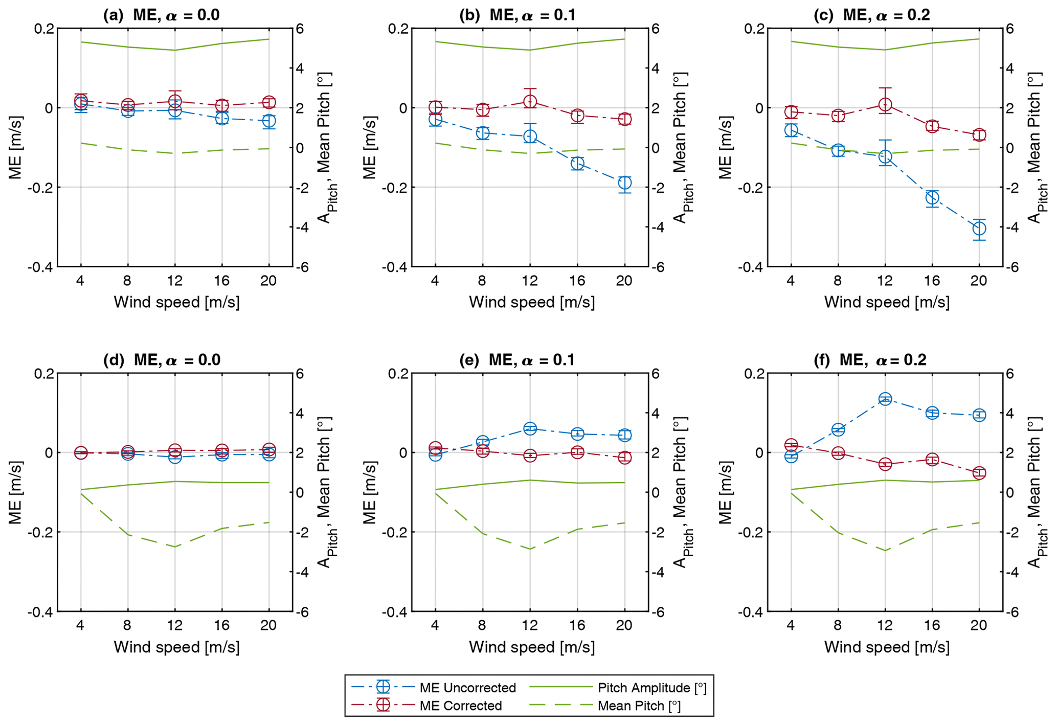
Figure 11 Mean errors of u wind speed component for FLOATGEN (a–c) and Windcrete (d–f) FOWT with and without correction for varying vertical shear exponents.

5.1 Model-based correction

Figure 11 shows the model-based correction results for simulated dynamics for the FLOATGEN (first row) and Windcrete (second row) FOWT. Before the correction, FLOATGEN shows negative mean errors in u-component wind speed, which increase with wind speed. This pattern is more pronounced under wind conditions with high vertical shear values. This behavior can be explained by the dynamic characteristics of FLOATGEN. As a barge-type floater, FLOATGEN shows insignificant mean pitch angles for the given conditions. On the other hand, floater pitch amplitudes show relatively high values for the given wave condition. Consequently, the negative effect of pitch movement is predominant. The model-based correction approach is able to reduce the ME significantly, resulting in ME below 0.1 m s⁻¹ or 0.5 %.

Table 6 Parameter space wave conditions, where H_s is the significant wave height, and T_p is the peak wave period.

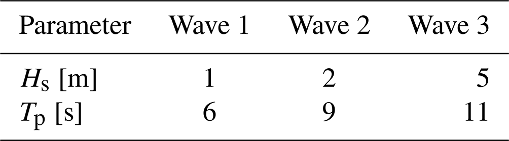
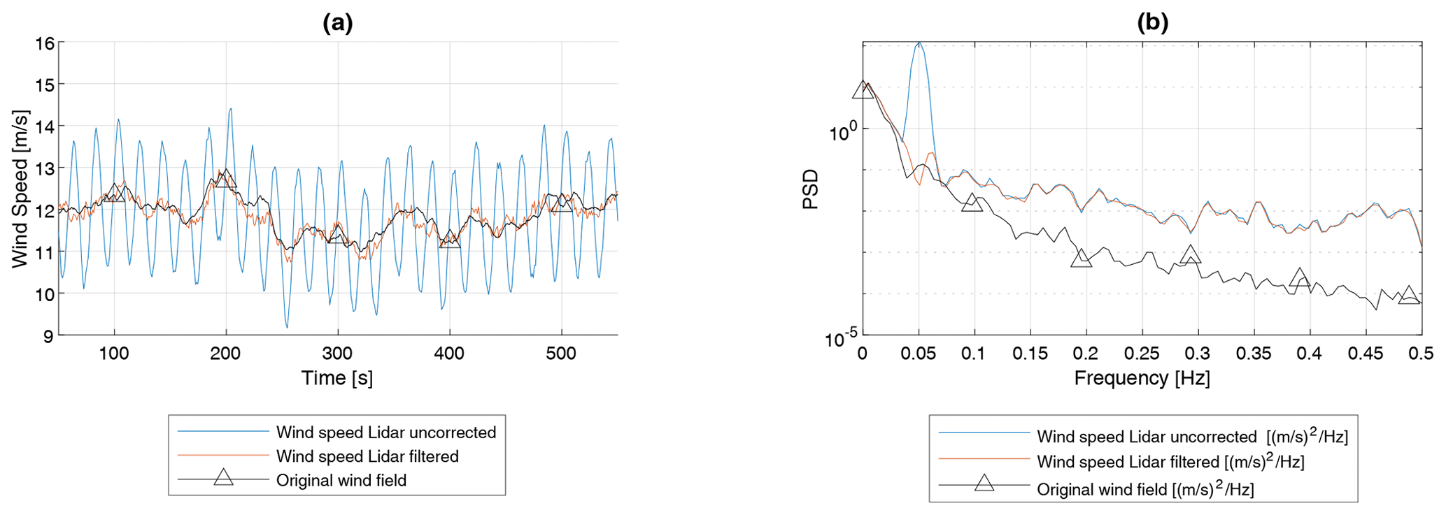
Figure 12 (a) Time series example of lidar-estimated u-component wind speed, frequency-corrected lidar u-component wind speed estimate, and reference wind speed of the input wind field. (b) Power spectral density of lidar-estimated u-component wind speed and frequency-corrected lidar u-component wind speed estimate. Dynamics parameters: U_ref = 12 m s⁻¹, A_β = 3^∘, T_β = 20 s, A_ψ = 0^∘, A_γ = 0^∘, and A_heave = 0 m.

The Windcrete FOWT model shows a different behavior. The mean error of the u-component wind speed before correction increases with the wind speedup to the rated wind speed of the turbine and slightly decreases for the above-rated wind conditions. The effect is more pronounced for high vertical shear conditions. The spar-type floater only shows small pitch amplitudes, below 1^∘, for the given wind and wave conditions. In contrast to FLOATGEN, the mean pitch angle shows relatively high values, especially at rated wind speed. Consequently, the positive effect of upward-shifted lidar focus points is predominant. In this case, the model-based correction approach can reduce the mean error significantly over the full wind speed range. The remaining MEs are below 0.1 m s⁻¹ or 0.5 %.

5.2 Frequency filtering

We first test the filtering approach using the lidar simulation framework ViConDAR for a random realization of a synthetic turbulent wind field with prescribed floater dynamics.

Figure 12 shows an exemplary time series plot of lidar-estimated u-component wind speed with and without application of the frequency filter. Additionally, the u-component wind speed component of the original wind field averaged over the rotor plane is shown as a reference. Since the floater pitch frequency is defined by only one frequency in this case, a narrow peak in the resulting PSD of the lidar-measured u-component is observed. The application of the bandstop filter corrects the pitch-induced fluctuations accurately.

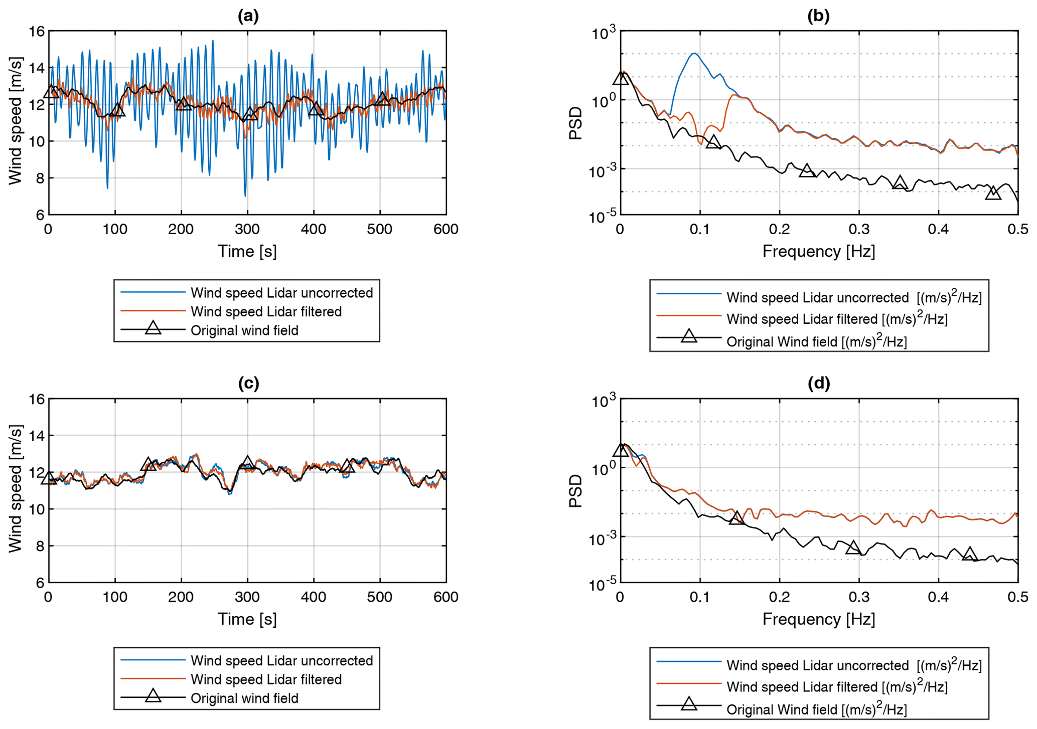
Figure 13 Time series and PSD of simulated lidar wind speed estimate with and without frequency correction for wave case 3 (see Table 6). (a, b) FLOATGEN and (c, d)Windcrete.

In Fig. 13, example time series and corresponding PSD plots for simulated lidar measurements on the FLOATGEN and Windcrete FOWT before and after the application of the bandstop filter are shown. As a reference, the wind speed average over the rotor plane is shown. The uncorrected measurements for FLOATGEN are characterized by periodic fluctuations caused by the floater's response to wave excitation. Application of the frequency filter reduces the fluctuations significantly. For the Windcrete FOWT, no clear influence of pitch motion can be observed in the time series and the corresponding PSD. Consequently, application of the frequency filtering cannot reduce the error between the lidar-measured wind speed and the full wind field reference. The reference PSD of the original wind field represents an average over all points in the rotor plane. Therefore, the spectrum lies below the lidar-estimated spectra. It should be noted that the lidar spectrum does contain the combined effect of probe volume averaging and cross contamination due to spatially separated measurement volumes.

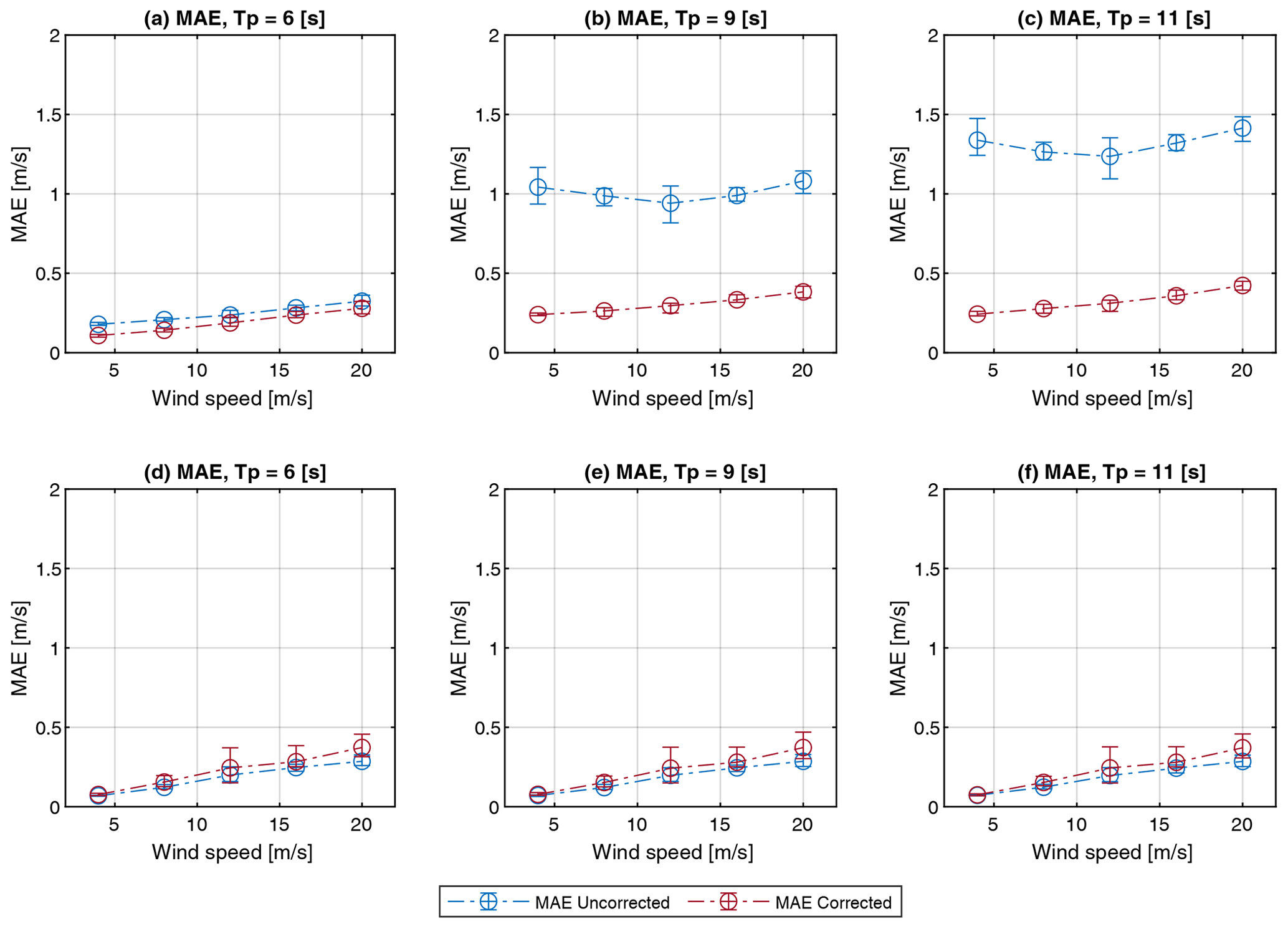
Figure 14 MAE of u wind speed component for FLOATGEN (a–c) and Windcrete (d–f) FOWT with and without correction for varying wave periods and vertical shear exponent of α=0.1.

Figure 14 shows the MAE results of the frequency-filter-based correction approach for simulated dynamics of FLOATGEN (first row) and Windcrete (second row) FOWT. For FLOATGEN, the pitch motion of the floater is mainly determined by the wave conditions with high pitch excitation for wave frequencies, close to the natural pitch frequency of the floater at 0.1 Hz. The frequency filtering of the present floater pitch frequency can significantly reduce the MAE.

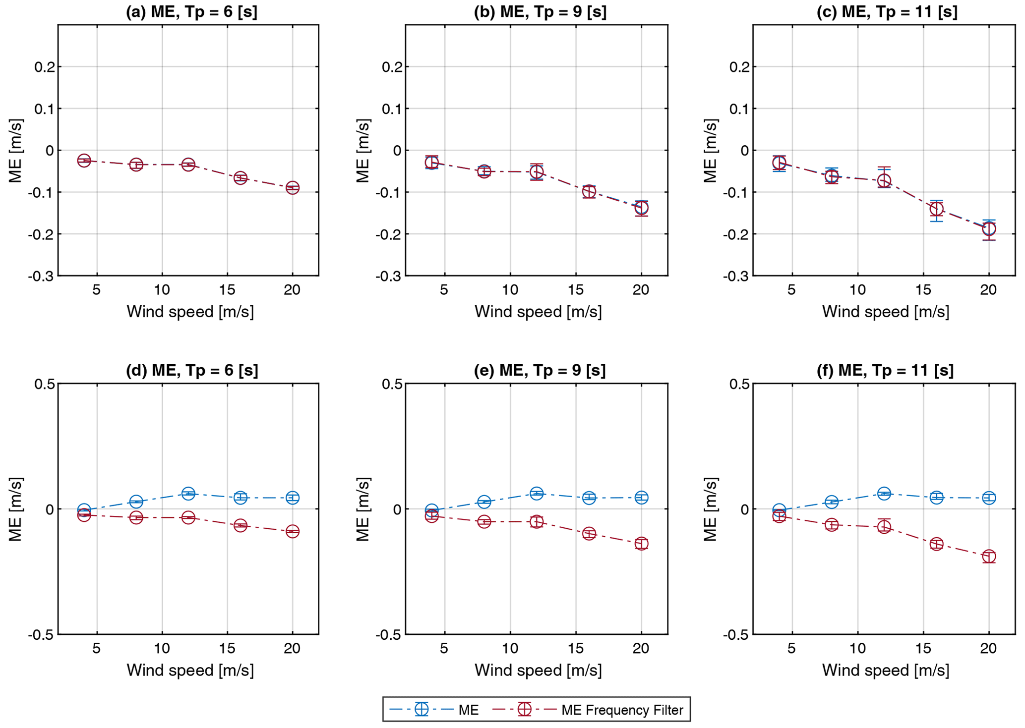
Figure 15 ME of u wind speed component for FLOATGEN  (a–c) and Windcrete (d–f) FOWT with and without application of frequency filter. Vertical shear exponent α=0.1.

For the given wind and wave conditions the Windcrete floater shows very small pitch excitation, resulting in small translational velocities of the nacelle and no significant peak in the frequency spectrum. In this case, the MAE is not affected by the frequency filtering approach. On the contrary, the MAE of the filtered lidar wind speed estimates is slightly higher compared to the uncorrected value because the applied frequency acts on the measured wind field spectrum itself. Thus, not only motion-induced frequency components are filtered. MAE values are not significantly influenced by wave conditions because of the small dependency between floater pitch response and different wave conditions.

Besides MAE, the second metric used to evaluate the performance of frequency filtering is ME. While for FLOATGEN, filtering of the pitch frequency does not introduce additional bias, for Windcrete bias of up to 0.2 m s⁻¹ is introduced in the time series. A comparison of ME before and after the application of the frequency filter is shown in Fig. 15. The MAE and ME results of this simulation study show that the proposed frequency filtering approach for motion correction is able to reduce MAE while not introducing bias. This applies only to floaters that cause a distinct peak around the pitch frequency of the floater in the frequency spectrum of the lidar wind speed measurements.

6 Discussion

The motion influence on nacelle-based lidar measurements was investigated with two different models. The introduced analytical model for the estimation of uncertainties and bias introduces several novelties and benefits compared to already-existing lidar simulation and uncertainty quantification frameworks.

First, it specifically addresses nacelle-based lidar systems on floating wind turbines for which very limited academic and industry experience exists, and uncertainty quantification is crucial for the application in various use cases. The advantage of this model over other, already available simulation tools lies mainly in its simplicity. The assumption of a power-law wind profile with no representation of turbulence does not require the generation of synthetic turbulent wind fields. The representation of floater dynamics in terms of frequency and amplitude parameters of the individual DOF avoids the need for numerical aeroelastic turbine-floater simulations. Thus, it allows an efficient estimation of motion-induced uncertainties and biases based on basic design parameters of the FOWT concept and the lidar configuration. In this way, expensive computational numerical simulation can be avoided, while still considering the most relevant effects of floater motion on the measurement. Based on these estimations and the intended use of the lidar measurements, decisions about correction approaches can be facilitated. As shown in Sect. 5.1 the use of model results for bias correction of measurements also shows additional potential for future use of the model.

The numerical model is more sophisticated and considers several characteristics which are neglected by the analytical model. In particular, it uses synthetic turbulent wind fields to account for the turbulent nature of real wind fields. Additionally, the probe-volume-averaging effect of lidar measurements is considered. The lidar setup is represented in a more realistic way, considering the temporal relation between the individual LOS measurements. A comparison of the results from the analytical and numerical models shows good agreement between both models. This indicates that the combined effect of turbulence, probe volume averaging, and time relation between the LOS measurements is small. The individual influence of these characteristics cannot be derived from our results, since no sensitivity study was conducted. However, comparing the results of the analytical and numerical model, we find good agreements between the two models, which in general gives confidence in the quantification of uncertainties. Based on a parametric study it was found that the most influential floater DOF for nacelle-based lidar measurement is the pitch displacement, leading to different effects relevant to different timescales. For time-averaged measurements, the pitch motion in combination with a vertical shear wind profile lead to an underestimation of wind speed. For FOWT configurations, operating at a non-zero mean pitch angle, shifted measurement positions in combination with a vertical shear profile lead to an overestimation of wind speed. Instantaneous wind speed measurements are mostly influenced by translational velocities of the nacelle, which are also caused by the rotational pitch movement of the floater. Two different approaches for the correction of these effects were introduced and tested using the numerical lidar simulation framework. The model-based bias correction approach is using bias estimates from the analytical model to calculate correction values as a function of pitch amplitude, frequency, and present shear conditions.

For the testing case using prescribed dynamics based on amplitude and frequency parameters, the correction approach yields very accurate results. Here, it should be noted that the analytical and numerical model use the same dynamics inputs. In reality, the modeled floater dynamics of the analytical model might not exactly represent the real floater dynamics. Also, the parameters determining the correction value for every 10 min are not constant for real floaters and need to be averaged, which adds uncertainties. However, the testing cases with the aeroelastic simulation of a spar-type and barge-type FOWT with very different pitch characteristics still yield good results with remaining mean errors of below 0.1 m s⁻¹. For all testing cases, it is assumed that the parameters necessary for the determination of correction values can be measured accurately. In reality, the determination of these parameters (mean pitch angle and pitch amplitude) would rely on inclination measurements, which could add uncertainty to the corrected wind speed estimates. A sensitivity study, quantifying the effect of these uncertainties, and further verification with real measurements are needed before the application of the methodology.

For higher pitch periods, translational velocities of the nacelle caused by floater pitch motions are not increasing the MEA significantly. Thus, the MEA is not predominantly determined by the pitch motion of the floater. Filtering of these frequencies yields increased MAEs, since relevant parts of the wind field spectrum are filtered out. Here, it should also be mentioned that the pitch frequency is assumed to be exactly known for each simulation run and not changing over time, which does not accurately represent the behavior of FOWTs under varying environmental conditions.

The testing cases using the simulated dynamics from FLOATGEN and Windcrete FOWT confirm the findings of the idealized conditions. For FLOATGEN, which has a relatively low natural pitch period of around 11 s and high pitch amplitudes, the MEA is predominantly determined by the pitch motion of the floater. Here, the MAE can be reduced significantly using the filtering approach. For Windcrete, with a natural pitch period of around 50 s and smaller pitch amplitudes, the filtering approach does not yield satisfactory results. For applications on real measurement data, the filtering frequencies need to be determined through measurements, e.g., based on a peak detection algorithm, which might introduce additional uncertainties. Therefore, verification of the method with real measurements is necessary.

7 Conclusions

In this study, we analyzed motion-induced effects on lidar measurements from forward-looking nacelle-mounted lidars on FOWT. For this analysis, we introduced a new analytical model for the estimation of uncertainty and bias in lidar-estimated wind speed. FOWT dynamics are modeled using amplitudes and periods of floater DOF in yaw, pitch, roll, and heave directions. The deterministic wind field is modeled by a simple power-law profile. Further, we applied the GUM methodology to derive combined uncertainties in the LOS measurements and in the reconstructed WFC. To verify the model outputs we compared the results to uncertainties derived with the numerical lidar simulation framework ViConDAR. This lidar simulation follows a more detailed modeling approach, in particular taking into account turbulent wind fields.

Results of a parametric study showed that the uncertainty of lidar-estimated wind speed estimates is mainly caused by the fore–aft motion of the lidar resulting from the pitch displacement of the floater. Therefore, the uncertainty is heavily dependent on the amplitude and the frequency of the pitch motion. The estimated bias in 10 min averaged wind speed is mainly influenced by the mean pitch angle of the floater, the pitch amplitude, and the vertical shear of the wind field.

Further, we introduced two approaches for the correction of motion-induced effects. We used the analytical model to derive a look-up table of correction values for 10 min averaged wind speed measurements. Testing of the approach with simulated dynamics from two different FOWT concepts showed good results. The remaining mean errors between simulated lidar measurements and input wind fields were found to be below 0.1 m s⁻¹ for both FOWT models. We used a frequency filter to correct fluctuations caused by floater pitch motions in instantaneous measurements. The correction can reduce the MAE in lidar wind speed estimates under certain conditions. The frequency filtering yields good results for dynamic conditions characterized by harmonic pitch oscillation with low pitch periods and high pitch amplitudes. For dynamic conditions characterized by varying pitch oscillation or high pitch periods and low amplitudes, the frequency filtering cannot reduce MEA in lidar wind speed estimates.

Appendix A

A1 Analytical estimation of uncertainty in wind field characteristics

Following the GUM methodology for expression of uncertainty (Sommer and Siebert, 2004), the total uncertainty of $y=f(x_{\mathrm{1}},x_{\mathrm{2}},\mathrm{\dots },x_n)$ with n uncorrelated input quantities xi is given by

$$\begin{array}{}\text{(A1)}& U_y^{\mathrm{2}}=\sum _{i=\mathrm{1}}^n\left({{\displaystyle \frac{\mathit{\delta }f}{\mathit{\delta }{x}_i}}}^{\mathrm{2}}\right)U_{x,i}^{\mathrm{2}},\end{array}$$

where U_x,i is the standard uncertainty of input quantity x_i.

Accordingly the total uncertainty in the LOS measurements, induced by floater dynamics, is given by

$$\begin{array}{}\text{(A2)}& U_{{\mathit{v}}_{\text{los}}}=\sqrt{\begin{array}{l}{\left(\frac{\mathit{\delta }{\mathit{v}}_{\text{los}}}{\mathit{\delta }\mathit{\psi }}\right)}^{\mathrm{2}}{U}_{\mathit{\psi }}^{\mathrm{2}}+{\left(\frac{\mathit{\delta }{\mathit{v}}_{\text{los}}}{\mathit{\delta }\mathit{\beta }}\right)}^{\mathrm{2}}{U}_{\mathit{\beta }}^{\mathrm{2}}+{\left(\frac{\mathit{\delta }{\mathit{v}}_{\text{los}}}{\mathit{\delta }\mathit{\gamma }}\right)}^{\mathrm{2}}{U}_{\mathit{\gamma }}^{\mathrm{2}}\\ +{\left(\frac{\mathit{\delta }{\mathit{v}}_{\text{los}}}{\mathit{\delta }{h}_{\text{heave}}}\right)}^{\mathrm{2}}{U}_{h_{\text{heave}}}^{\mathrm{2}}+{\frac{\mathit{\delta }{\mathit{v}}_{\text{los}}}{\mathit{\delta }{x}_{\text{vel}}}}^{\mathrm{2}}{U}_{x_{\text{vel}}}^{\mathrm{2}}\end{array}},\end{array}$$

where $U_{\mathit{\psi }},U_{\mathit{\beta }},U_{\mathit{\gamma }},U_{h_{\text{heave}}}$, and $U_{x_{\text{vel}}}$ are the standard uncertainties of input quantities. The formulation in Eq. (A2) assumes that the considered input quantities are uncorrelated. As the input quantities represent the dynamics of the floater, which are closely connected to wave forces acting on the floater, they are modeled as harmonic oscillations. Following Sommer and Siebert (2004), the standard uncertainties of this type of input quantities are given by

$$\begin{array}{}\text{(A3)}& U_a={\displaystyle \frac{\mathrm{\Delta }a}{\sqrt{\mathrm{2}}}},\end{array}$$

where a_i is the amplitude of the assumed oscillation of the input quantity i. The derivatives in Eq. (A2) are the partial derivatives of Eq. (9) with respect to the considered input quantities. The solutions of the partial derivatives can be found in Appendix A4.

A2 Uncertainty propagation through wind field reconstruction

In this section, we derive uncertainties in the reconstructed wind field characteristics based on previously derived LOS uncertainties. Since the lidar is only able to measure the wind speed in the line-of-sight direction, wind field characteristics including the horizontal wind speed components need to be reconstructed from the LOS measurements. It is not possible to reconstruct the three-dimensional wind vector from a single LOS measurement unambiguously. Different approaches to this problem like the velocity–azimuth display technique introduced by Browning and Wexler (1968) are discussed in the literature. Other approaches combine several LOS measurements and use assumptions about spatial and temporal correlations between the measurements to reconstruct the wind field characteristics (see, e.g., Borraccino et al., 2017).

For the analytical derivation of uncertainty, we employ a simple wind field reconstruction algorithm that assumes the v and w components of the wind field to be zero. Under this assumption, all contributions to the measured radial velocity are attributed to the u component of the wind field, which can lead to an overestimation of this component. The uncertainty related to this effect increases with growing magnitudes of v and w components. The implementation of other reconstruction approaches is possible but requires modifying the corresponding partial derivatives. The reconstructed u component of the wind speed at each beam is given by

$$\begin{array}{}\text{(A4)}& u_i={\displaystyle \frac{v_{\text{los},i}}{x_{\mathrm{L},i}{r}_i}},\end{array}$$

with v_los,i being the LOS wind speed of beam 1 to 4, x_L,i being the focus point x coordinate of beam i, and r_i being the measurement distance. Further we combine the measurements of all four beams by averaging the wind speed estimates of the individual beams.

Thus, the reconstructed wind speed component u_rec is given by

$$\begin{array}{}\text{(A5)}& u_{\text{rec}}={\displaystyle \frac{\mathrm{1}}{\mathrm{4}}}\cdot \left({\displaystyle \frac{v_{\text{los},\mathrm{1}}}{x_{\mathrm{L},\mathrm{1}}{r}_{\mathrm{1}}}}+{\displaystyle \frac{v_{\text{los},\mathrm{2}}}{x_{\mathrm{L},\mathrm{2}}{r}_{\mathrm{2}}}}+{\displaystyle \frac{v_{\text{los},\mathrm{3}}}{x_{\mathrm{L},\mathrm{3}}{r}_{\mathrm{3}}}}+{\displaystyle \frac{v_{\text{los},\mathrm{4}}}{x_{\mathrm{L},\mathrm{4}}{r}_{\mathrm{4}}}}\right).\end{array}$$

Again, the uncertainty of the reconstructed horizontal wind speed components can be estimated by combining the standard of uncertainties of the input quantities by following the GUM methodology. The combined uncertainty of n correlated input quantities is given by

$$\begin{array}{}\text{(A6)}& U_y^{\mathrm{2}}=\sum _{i=\mathrm{1}}^{\mathrm{4}}{{\displaystyle \frac{\mathit{\delta }f}{\mathit{\delta }{x}_i}}}^{\mathrm{2}}\cdot U_i^{\mathrm{2}}+\mathrm{2}\sum _{i=\mathrm{1}}^{N-\mathrm{1}}\sum _{j=i+\mathrm{1}}^N{\displaystyle \frac{\mathit{\delta }f}{\mathit{\delta }{x}_i}}{\displaystyle \frac{\mathit{\delta }f}{\mathit{\delta }{x}_j}}{U}_i{U}_j{r}_{i,j},\end{array}$$

where r_i,j is the correlation coefficient of beam i and j. Considering Eq. (A5), the reconstructed wind speed component u_rec is a function of the four LOS velocities. Thus the total uncertainty of u_rec given by

$$\begin{array}{}\text{(A7)}& \begin{array}{rl}{U}_{u_{\text{rec}}}^{\mathrm{2}}& =\sum _{i=\mathrm{1}}^n{{\displaystyle \frac{\mathit{\delta }u}{\mathit{\delta }{v}_{\text{los},i}}}}^{\mathrm{2}}\cdot U_{\text{los},i}^{\mathrm{2}}\\ & +\mathrm{2}\sum _{i=\mathrm{1}}^{N-\mathrm{1}}\sum _{j=i+\mathrm{1}}^N{\displaystyle \frac{\mathit{\delta }u}{\mathit{\delta }{v}_{\text{los},i}}}{\displaystyle \frac{\mathit{\delta }u}{\mathit{\delta }{v}_{\text{los},j}}}{U}_{\text{los},i}{U}_{\text{los},j}{r}_{i,j},\end{array}\end{array}$$

where U_los,i is the standard uncertainty of beam i as calculated in Eq. (A2). In this case, the LOS velocities of the four beams cannot be assumed to be uncorrelated. The correlation is considered by the correlation coefficient r_i,j of the LOS velocities of beam i and j. The partial derivatives can be found in Appendix A4.

The correlation coefficients between the LOS measurements of the individual beams are needed as a parameter for the calculation of uncertainty of reconstructed wind field characteristics. They are influenced by the changing LOS directions and the position of focus points in space and the assumed wind field. Thus, correlation coefficients are dependent on the set of dynamic input parameters and the phasing between the single DOF. In the model, the correlation coefficients are calculated for the present set of model input parameters. This is done by evaluating Eq. (9) over time for each LOS and calculating the correlation between the resulting LOS time series.

A3 Analytical estimation of bias

The lidar measurement model introduced in Sect. 2.2 is also used to estimate systematic biases in reconstructed wind field characteristics that occur due to floater dynamics. Using Eq. (9), which combines the temporal evolution of all dynamic input quantities, the LOS velocity is calculated for a defined parameter space over a defined time span. Further, the wind field reconstruction approach introduced before is applied to calculate the horizontal wind speed component u_rec. The bias of the reconstructed u-component wind speed is calculated by

$$\begin{array}{}\text{(A8)}& {\mathrm{Bias}}_u=u_{\text{ref}}-u_{\text{rec,mean}},\end{array}$$

where u_ref is the reference wind speed, and u_rec,mean is the mean value of the reconstructed wind speed component. The reference wind speed is calculated as the average over a rotor plane. The rotor diameter for this hypothetical rotor is chosen to be d_rotor = 150 m. The results of the bias estimation are very sensitive to the exact calculation procedure of the reference value. Therefore, to make the results comparable to the numerical model results, the calculation procedure is the same as in the numerical model. In the numerical model, the u wind speed components of all grid points of the synthetic wind field which are within the rotor plane are averaged. For the reference values u_ref of the analytical model, the wind speed components of the same grid points are calculated according to the assumed power-law wind profile. The average of these points is taken to calculate u_ref.

Equation (9) combines the temporal evolution of all dynamic input quantities. Therefore, different effects can potentially influence the estimation of bias. First, it must be ensured that the length of the time window of calculation is large enough to avoid any relevant influence of time window length on the bias estimation. Second, the phasing between the individual dynamics input quantities could influence the bias estimation.

Figure A1a shows the standard deviation within 100 realizations of the bias estimation of the wind speed u component for one set of input parameters as a function of time window length. The phasing of input dynamics (yaw, pitch, roll, and heave) is randomized for each realization. It can be seen that the standard deviation is fluctuating over the time window length, depending on the ratio between time window length and dynamics frequencies, with minima for time window lengths being multiples of dynamics frequencies. This effect is small for longer time window lengths where the averaging period is 1 order of magnitude higher than the period of input dynamics. The remaining fluctuation in standard deviation for a time window length of 600 s is small and can be neglected. However, the standard deviation is not converging to 0, since the random phasing between the individual dynamics input quantities is part of the standard deviation. Therefore, several random realizations with a time window length of 600 s are averaged. Figure A1b shows the standard deviation of averaged bias estimates as a function of the number of random realizations, averaged for one bias estimate. For the remainder of the work, all bias estimates of the analytical model are calculated for a time window length of 600 s and averaged over 10 random realizations.

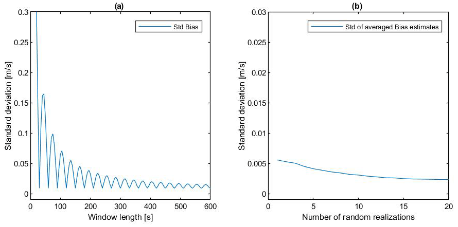
Figure A1 (a) Standard deviation of bias estimation within 100 random realization over the time window length. (b) Standard deviation of averaged bias estimations over a number of averaged random realizations with a time window length of 600 s.

A4 Partial derivatives

$$\begin{array}{}\text{(A9)}& \begin{array}{rl}{\displaystyle \frac{\mathit{\delta }{\mathit{v}}_{\text{los}}}{\mathit{\delta }\mathit{\psi }}}& =-V_{\text{ref}}{\left({\displaystyle \frac{z_{\mathrm{L}}+h_{\text{lidar}}+h_{\text{heave}}}{H_{\text{ref}}}}\right)}^{\mathit{\alpha }}\\ & \times \left(\sin \mathit{\phi }\right(x_{\mathrm{L}}\sin \mathit{\psi }+y_{\mathrm{L}}\cos \mathit{\psi }\left)\right)\\ & +\cos \mathit{\psi }(y_{\mathrm{L}}\sin \mathit{\psi }-x_{\mathrm{L}}\cos \mathit{\psi }),\end{array}\end{array}$$

$$\begin{array}{}\text{(A10)}& {\displaystyle }\begin{array}{rl}{\displaystyle \frac{\mathit{\delta }{\mathit{v}}_{\text{los}}}{\mathit{\delta }\mathit{\beta }}}& ={\displaystyle \frac{\begin{array}{c}\mathit{\alpha }{V}_{\text{ref}}(-x_{\mathrm{L}}\cos \mathit{\beta }-z_{\mathrm{L}}\sin \mathit{\beta })\\ \times \left(\sin \mathit{\phi }\right(x_{\mathrm{L}}\cos \mathit{\beta }+z_{\mathrm{L}}\sin \mathit{\beta })\\ +y_{\mathrm{L}}\cos \mathit{\phi }){\left(\frac{h_{\text{lidar}}+h_{\text{heave}}-x_{\mathrm{L}}\sin \mathit{\beta }+z_{\mathrm{L}}\cos \mathit{\beta }}{H_{\text{ref}}}\right)}^{\mathit{\alpha }-\mathrm{1}}\end{array}}{H_{\text{ref}}}}\\ & +V_{\text{ref}}\sin \mathit{\phi }(z_{\mathrm{L}}\cos \mathit{\beta }-x_{\mathrm{L}}\sin \mathit{\beta })\\ & \times {\left({\displaystyle \frac{h_{\text{lidar}}+h_{\text{heave}}-x_{\mathrm{L}}\sin \mathit{\beta }+z_{\mathrm{L}}\cos \mathit{\beta }}{H_{\text{ref}}}}\right)}^{\mathit{\alpha }},\end{array}\text{(A11)}& {\displaystyle }\begin{array}{rl}{\displaystyle \frac{\mathit{\delta }{\mathit{v}}_{\text{los}}}{\mathit{\delta }\mathit{\gamma }}}& ={\displaystyle \frac{\begin{array}{c}\mathit{\alpha }{V}_{\text{ref}}(y_{\mathrm{L}}\cos \mathit{\gamma }-z_{\mathrm{L}}\sin \mathit{\gamma })\\ \times (x_{\mathrm{L}}\sin \mathit{\phi }+\cos \mathit{\phi }(y_{\mathrm{L}}\cos \mathit{\gamma }-z_{\mathrm{L}}\sin \mathit{\gamma })\\ \times {\left(\frac{h_{\text{lidar}}+h_{\text{heave}}+x_{\mathrm{L}}\sin \mathit{\gamma }+z_{\mathrm{L}}\cos \mathit{\gamma }}{H_{\text{ref}}}\right)}^{\mathit{\alpha }-\mathrm{1}}\end{array}}{H_{\text{ref}}}}\\ & +V_{\text{ref}}\cos \mathit{\phi }(-y_{\mathrm{L}}\sin \mathit{\gamma }-z_{\mathrm{L}}\cos \mathit{\gamma })\\ & \times {\left({\displaystyle \frac{h_{\text{lidar}}+h_{\text{heave}}+y_{\mathrm{L}}\sin \mathit{\gamma }+z_{\mathrm{L}}\cos \mathit{\gamma }}{H_{\text{ref}}}}\right)}^{\mathit{\alpha }},\end{array}\text{(A12)}& {\displaystyle }{\displaystyle \frac{\mathit{\delta }{\mathit{v}}_{\text{los}}}{\mathit{\delta }{h}_{\text{heave}}}}={\displaystyle \frac{\mathit{\alpha }{V}_{\text{ref}}{\left(\frac{h_{\text{heave}}+h_{\text{lidar}}+z_{\mathrm{L}}}{H_{\text{ref}}}\right)}^{\mathit{\alpha }}(x_{\mathrm{L}}\sin \mathit{\phi }+y_{\mathrm{L}}\cos \mathit{\phi })}{h_{\text{heave}}+h_{\text{lidar}}+z_{\mathrm{L}}}},\end{array}$$

$$\begin{array}{}\text{(A13)}& {\displaystyle \frac{\mathit{\delta }{\mathit{v}}_{\text{los}}}{\mathit{\delta }{x}_{\text{vel}}}}=x_I{\displaystyle \frac{\mathit{\delta }{\mathit{v}}_{\text{los}}}{\mathit{\delta }{x}_{\text{vel}}}}=y_I{\displaystyle \frac{\mathit{\delta }{\mathit{v}}_{\text{los}}}{\mathit{\delta }{z}_{\text{vel}}}}=z_I,\text{(A14)}& {\displaystyle \frac{\mathit{\delta }u}{\mathit{\delta }{v}_{\text{los},i}}}={\displaystyle \frac{\mathrm{1}}{\mathrm{4}}}{\displaystyle \frac{\mathrm{1}}{x_{\mathrm{L},i}}}.\end{array}$$

A5 Rotation matrices

The rotation matrix is given by

$$\begin{array}{}\text{(A15)}& \begin{array}{rl}\mathbf{R}(\mathit{\psi },\mathit{\beta },\mathit{\gamma })& =\left[\begin{array}{ccc}\cos \mathit{\psi }& -\sin \mathit{\psi }& \mathrm{0}\\ \sin \mathit{\psi }& \cos \mathit{\psi }& \mathrm{0}\\ \mathrm{0}& \mathrm{0}& \mathrm{1}\end{array}\right]\\ & \times \left[\begin{array}{ccc}\cos \mathit{\beta }& \mathrm{0}& \sin \mathit{\beta }\\ \mathrm{0}& \mathrm{1}& \mathrm{0}\\ -\sin \mathit{\beta }& \mathrm{0}& \cos \mathit{\beta }\end{array}\right]\\ & \times \left[\begin{array}{ccc}\mathrm{1}& \mathrm{0}& \mathrm{0}\\ \mathrm{0}& \cos \mathit{\gamma }& -\sin \mathit{\gamma }\\ \mathrm{0}& \sin \mathit{\gamma }& \cos \mathit{\gamma }\end{array}\right].\end{array}\end{array}$$