the Creative Commons Attribution 4.0 License.
the Creative Commons Attribution 4.0 License.
 | 13 Jun 2023
From shear to veer: theory, statistics, and practical application
Maarten Paul van der Laan
In the past several years, wind veer – sometimes called “directional shear” – has begun to attract attention due to its effects on wind turbines and their production, particularly as the length of manufactured turbine blades has increased. Meanwhile, applicable meteorological theory has not progressed significantly beyond idealized cases for decades, though veer's effect on the wind speed profile has been recently revisited. On the other hand the shear exponent (α) is commonly used in wind energy for vertical extrapolation of mean wind speeds, as well as being a key parameter for wind turbine load calculations and design standards.
In this work we connect the oft-used shear exponent with veer, both theoretically and for practical use. We derive relations for wind veer from the equations of motion, finding the veer to be composed of separate contributions from shear and vertical gradients of crosswind stress. Following from the theoretical derivations, which are neither limited to the surface layer nor constrained by assumptions about mixing length or turbulent diffusivities, we establish simplified relations between the wind veer and shear exponent for practical use in wind energy. We also elucidate the source of commonly observed stress–shear misalignment and its contribution to veer, noting that our new forms allow for such misalignment. The connection between shear and veer is further explored through analysis of one-dimensional (single-column) Reynolds-averaged Navier–Stokes solutions, where we confirm our theoretical derivations as well as the dependence of mean shear and veer on surface roughness and atmospheric boundary layer depth in terms of respective Rossby numbers.
Finally we investigate the observed behavior of shear and veer across different sites and flow regimes (including forested, offshore, and hilly terrain cases) over heights corresponding to multi-megawatt wind turbine rotors, also considering the effects of atmospheric stability. From this we find empirical forms for the probability distribution of veer during high-veer (stable) conditions and for the variability in veer conditioned on wind speed. Analyzing observed joint probability distributions of α and veer, we compare the two simplified forms we derived earlier and adapt them to ultimately arrive at more universally applicable equations to predict the mean veer in terms of observed (i.e., conditioned on) shear exponent; lastly, the limitations, applicability, and behavior of these forms are discussed along with their use and further developments for both meteorology and wind energy.
- Article
(4618 KB) - Full-text XML
- BibTeX
- EndNote


The shear exponent has generally not been used or accepted by meteorologists, as it does not (directly) relate to the physics of atmospheric flow nor to the most important boundary condition – the surface. Regarding the latter, in contrast with similarity theory (Monin and Obukhov, 1954), the shear exponent does not contain explicit information about the surface roughness. However, the shear exponent can be related to surface properties in a generalized way, as well as to turbulent kinetic energy and atmospheric stability (buoyancy) as shown by, e.g., Kelly et al. (2014a). This is particularly useful above the atmospheric surface layer (ASL), where micrometeorological theory based on ASL assumptions fails – and where the effects of the surface are neither dominant nor simple enough to be characterized through accepted ASL parameterizations. As practiced in the wind energy resource assessment community for decades, the shear exponent can thus be preferable over similarity theory for use in vertical extrapolation (Irwin, 1979; Mikhail, 1985; Petersen et al., 1998) with quantification of uncertainty in its use more recently reinforcing this (Triviño, 2017; Kelly et al., 2019b). Shear is also a key parameter for flow characterization towards load simulations, being seen to systematically affect various turbine loads (e.g., Dimitrov et al., 2018; Robertson et al., 2019).
Veer has received much less attention than shear, though its potential importance to wind energy has been noted more recently. In the meteorological literature, where veer is often labeled as “directional shear” or “turning”, Markowski and Richardson (2006) reviewed the distinction between veer and vertical gradients of wind speed, listing studies of meteorological phenomena that considered veer (though they focused on convective storms). While some works in meteorology have investigated veer, these have tended to focus on the angular difference between winds at the top of the atmospheric boundary layer (ABL) and the surface (e.g., Clarke, 1975; Brown et al., 2005; Grisogono, 2011; Lindvall and Svensson, 2019), and they are not generally suited for engineering applications. For wind energy, Murphy et al. (2020) looked at the veer (and shear) along with power production measured over a 6-month period, finding a minor but non-negligible effect of veer on power production for a utility-scale turbine. Gao et al. (2021) found positive veer over the upper half of a single (2.5 MW) clockwise-turning turbine rotor to reduce power production, opposite to and slightly larger than the corresponding effects of negative veer there; they also showed the rotor's lower-half veer was less significant than the upper half. Shu et al. (2020) examined measurements from a lidar offshore between islands southwest of Hong Kong, observing larger veer when hilly terrain was upstream compared to more open-sea conditions; they also noted seasonal variations. For power production, the veer was incorporated into rotor-equivalent wind speed (REWS) by Choukulkar et al. (2016), who found it to generally decrease production at two sites; Clack et al. (2016) found similar results from weather assimilation model output over the USA, along with higher production at night and lower power during daytime at most locations. Wind veer has also been examined with regard to its connection with the distortion and lateral-movement turbine wakes via measurements and simulations (e.g., Abkar et al., 2018; Brugger et al., 2019), also including yaw-misalignment effects (Hulsman et al., 2022; Narasimhan et al., 2022).
In this paper we investigate wind veer, showing its joint behaviors with and connection to shear and key parameters used to describe atmospheric boundary layer flow. In Sect. 2, after reviewing the expression of the shear exponent and its relation to stability and turbulence, we derive new relations for veer; we show veer to be composed of shear-driven and Coriolis-associated stress gradient contributions. The theoretical behavior of veer is also derived for canonical cases such as Ekman and surface-layer flow, as well as the effect of shear-stress misalignment on veer. Further, in Sect. 2.4 practical relations from micrometeorology are elucidated towards an evaluation of the expressions developed for veer. Section 3 includes an analysis of veer, exploring and connecting the developed relations to both computational modeling and observations. Section 3.1 gives Reynolds-averaged Navier–Stokes (RANS; mean) simulation results over flat terrain in neutral conditions for hundreds of combinations of surface Rossby number and ABL-depth Rossby number, showing the dependence of veer on the latter, as well as the counteracting behavior of veer's two primary components. Section 3.2 begins with an analysis of multi-year observations from six different flow regimes across four sites showing the statistical behavior of shear with stability and subsequently that of veer, also providing new empirical relations for the probability of occurrence of larger veer (due to the effect of stable conditions) and for the variability in veer with wind speed. The observational analysis concludes in Sect. 3.3 with simplified practical relations for veer based on observed shear, including a comparison with joint distributions of veer and shear across the six flows analyzed. Finally the results are summarily discussed and conclusions given, with ongoing and future work also described for the reader.
In this section we define the shear exponent and veer and then derive relations for veer in terms of shear and vertical gradients of stress, as mentioned in the previous paragraph. Section 2.3 provides a number of expressions for veer; this is done to facilitate its calculation and interpretation in the different coordinate systems typically considered in wind energy flow analyses, and we also include forms that are independent of coordinate system. Because coordinates aligned with the mean wind for a given height of interest (e.g., hub height) are commonly used in wind energy and because expressions for veer in such a coordinate system are simpler to express and calculate, we ultimately arrive at two forms in such a system (Eqs. 14 and 16); due to its robustness, one of these (Eq. 14) will later be shown in Sect. 3.3 to be further simplifiable and usable (as Eqs. 39 or 40) in comparison with measurements.
2.1 Shear exponent
Just as potential temperature – the buoyancy variable commonly used in meteorology – was labeled the “meteorologist's entropy” by Bohren and Albrecht (1998), one could call the shear exponent (α) the “wind engineer's phi-function”. Specifically this follows from the definition of shear exponent,
and the dimensionless wind speed gradient,
used in meteorology, where u*0 is the surface-layer friction velocity (square root of kinematic shear stress), κ=0.4 is the von Kármán constant, and z is the height coordinate1. Note that Eq. (1) is derived from the power-law expression for wind speed,
which is assumed to be valid over some extent around height zref, with Uref≡U(zref). The power-law (Eq. 3) with shear exponent (Eq. 1) has been used in wind engineering for decades (e.g., Irwin, 1979; Petersen et al., 1998) due to its simplicity and because it does not require any information other than the wind speed at two heights. Although Eqs. (1) and (2) might appear to be quite alike, one can see a phenomenological difference when comparing the wind speed profiles resulting from these relations. In Monin–Obukhov (M–O) theory Φm is a function of the stability which is proportional to surface heat flux H0 divided by , i.e., the reciprocal Obukhov length is , where T0 is the background temperature and g is the gravitational acceleration (Monin and Obukhov, 1954); the Φm function and corresponding M–O wind profile (which arises via integrating in Eq. (2) from a height equal to the roughness length z0 up to height z) thus require a number of assumptions and more information than the calculation of α via Eq. (1) or use of the power-law (Eq. 3). Monin–Obukhov wind profiles also require the surface roughness length (z0), while the friction velocity u*0 (and thus shear stress) is assumed to be constant in the surface layer where M–O theory is most valid2; further, the assumptions of stationarity and a uniform flat surface are implicit in the use of M–O theory. Following surface-layer theory one could write an equivalent shear exponent , where
is the M–O wind speed correction function; the analytic forms for Φm and Ψm differ in stable and unstable conditions and have been determined empirically in decades past (Businger et al., 1971; Carl et al., 1973; Li, 2021). But Monin–Obukhov similarity theory and its assumptions (such as constant u*), as well as established forms for Φm, fail above the surface layer3.
2.1.1 Relation to stability and turbulence
As shown by Kelly et al. (2014a), in horizontally homogeneous conditions the steady or mean balance of turbulent kinetic energy (TKE) can be written in terms of shear exponent as
for a given height z, where the streamwise direction is defined by the mean wind U(z) and we have suppressed z dependences for brevity; here 〈uw〉 is the turbulent horizontal momentum flux (kinematic stress), T is the total (turbulent plus pressure) transport, B is buoyant production, and ε is the viscous dissipation rate of TKE. We point out that Kelly et al. (2014a) ignored crosswind stress 〈vw〉 when deriving Eq. (4); however, it still shows that, e.g., shear will increase in stable conditions (B<0) and decrease in unstable conditions (B>0), as will be demonstrated using observations in Sect. 3.2; further, as we will see in Sect. 2.3, this is also related to the veer. Within the ASL under these conditions where M–O theory is valid and 〈vw〉→0, using the neutral value of dissipation rate as along with the dimensionless functions and (Kaimal and Finnigan, 1994), we can express a surface-layer version of Eq. (4) as
since by definition and ; here is the streamwise turbulence intensity. The dimensionless dissipation rate (M–O function) Φε≥1 is roughly in stable conditions and increases more weakly with in unstable conditions (Panofsky and Dutton, 1984; Kaimal and Finnigan, 1994); meanwhile the transport is negligible in stable conditions but ΦT>0 in unstable conditions (e.g., Wyngaard, 2010). Thus in stable conditions () one can see α is larger than in neutral conditions, while in unstable conditions α becomes smaller. Above the ASL this will also generally be the case, though analytic nondimensional forms become difficult to derive, while the flow becomes affected by more terrain upwind and associated inhomogeneities; furthermore in stable conditions the local stability (at a given z) becomes increasingly more important than surface-based (Derbyshire, 1990). As will be shown below, the most common and mean conditions at contemporary rotor heights qualitatively follow Eq. (5), but due to these and other non-ideal effects (e.g., nonstationary transients) large deviations can occur. We note that in this work we are not searching for analytical forms for α or surface-layer behavior; rather, we are concerned with how α relates to the veer, especially over heights corresponding to wind turbine rotors, a portion of which commonly extends beyond the ASL.
2.2 Veer
For the simplified general case of Coriolis-affected mean flow, we write the horizontal mean velocity vector {U,V} as a complex number, . For a mean wind direction defined at some height z, the veer can be defined as a directional shear through the wind direction:
In most of the micrometeorological literature, the mean wind direction is defined based on the surface stress (i.e., via the winds closest to the surface, so ). We follow this convention unless stated otherwise, as done for some expressions later in Sect. 2.3; one could also choose to define the coordinate system based on the geostrophic wind direction (e.g., Svensson and Holtslag, 2009).
As is classically known in micrometeorology (e.g., Hess and Garratt, 2002), the veer across the entire ABL depends primarily on the Coriolis parameter f (thus latitude), geostrophic wind speed , and surface roughness length z0 but is also affected by the ABL depth h and stability (as confirmed via Reynolds-averaged Navier–Stokes simulations by van der Laan et al., 2020). The veer across a fraction of the ABL will also depend on these parameters; thus for a given site and height, will have a distribution due to variations in these parameters. This will become clearer below as we examine the relationship between veer and shear.
The Coriolis-affected mean momentum balance can be written in the form
for stationary and horizontally homogeneous conditions (thus neglecting advection). Here the kinematic horizontal pressure gradient is also written like a velocity in complex form as . The mean stresses are dominated by vertical momentum transport 〈sw〉, where w denotes (turbulent) vertical velocity fluctuations and the horizontal velocity fluctuations.
At a given height z, taking the differential of Eq. (6) (recalling and using the chain rule) gives
here the superscript asterisk denotes a complex conjugate. Applying to Eqs. (7) and (8) and combining provides a basic expression for veer:
In the case of zero geostrophic shear (), if the coordinate system's x axis is defined by the mean wind direction at the height z where the veer is sought, then Eq. (9) can be written more simply as
Though Eqs. (9) and (10) are not directly very useful for relating veer to shear, since the shear is implicit in the stress terms (and one would need to know the profiles of horizontal stresses to use these equations), they do illustrate that the curvature of stress profiles and Coriolis effect are the basis for mean veer following Eq. (7) and also that geostrophic shear can further contribute to veer (e.g., due to baroclinity; see Hoxit, 1974; Arya and Wyngaard, 1975; Pedersen et al., 2013).
2.3 Relating veer to shear
Towards relating the veer to shear, one can alternately derive the veer by first taking the time derivative of Eq. (8); using the real and imaginary parts of Eq. (7), in the horizontally homogeneous limit (ignoring advection) one obtains a rate equation for mean wind direction:
The “turning” angle between geostrophic and mean wind directions (e.g., Wyngaard, 2010) arises through4
by taking of Eq. (6) or equivalently via Eq. (8). The geostrophic wind direction is defined as , and the “cross-isobar” angle, i.e., the turning over the whole ABL , is generally less than 45∘ (Grisogono, 2011)5; in a right-handed coordinate system, regardless of whether x is chosen to align with G or the surface-layer wind velocity UASL, the turning tends to γ>0 in the Northern Hemisphere6. Note that φ, and thus γ, can vary with height z (as can φG in baroclinic conditions).
Assuming statistical stationarity so that , the vertical derivative of Eq. (11) can be written most conveniently in terms of the deviation of dimensionless wind from streamwise; taking the vertical derivative of Eq. (11) if we again take (neglect baroclinity), then
As it is expressed in terms of angular differences γ, the equation above is independent of whether the coordinate system is defined at the surface or by the geostrophic wind. Equation (12) clearly separates the shear and stress–Coriolis contributions to veer. However, it can be simplified, and is most meaningful, if the coordinate system is defined at the height z for which it is applied; in practice the veer is typically calculated around hub height, from hub to tip, or between measurement and hub heights. Re-expressing Eq. (11) with the coordinate system defined by having x in the mean wind direction at height z so that S(z)=U(z)ex and , in the mean (for ) one has
where we use the shorthand notation 〈vw〉⟂ to denote the stress perpendicular to the mean flow at a given height. Taking the inverse cosine and subsequently the vertical derivative, noting that and while recalling , we get
here the subscript ∥ is used to remind us that 〈uw〉 is parallel to the flow at height z. Further, this coordinate system (Eq. 8) gives so that the part just becomes an additional veer term on the right-hand side; collecting the on the left side and rearranging we then obtain
As will be demonstrated in a later section, basically one sees from the numerator of Eq. (14) that the veer is comprised of a shear-associated part and a crosswind stress-curvature part; the denominator is basically 1 minus a few relatively small terms. The more generic form of veer, for an arbitrary coordinate system, also follows from Eq. (11):
We note that Eqs. (14) and (15) avoid the use of the turning (ageostrophic) angle γ, and subsequently nonlinear functions involving φG, which becomes apparent if one expands cos γ in Eqs. (12) or (13). However, one can see that there can be an angular dependence within the stress-related parts written above; when considered in coordinates defined with the x direction aligned with the mean wind at height z, in the general forms Eqs. (12) and (15), and can be written as cos φ and sin φ, respectively. Then from Eq. (12) and using , again in coordinates defined by , after some rearranging we arrive at an expression for veer like Eq. (14):
Compared to Eq. (14) this lacks a negative sign, but sin φG is negative and with a larger magnitude than the positive contribution to the denominator, ; this will become more apparent in the sections which follow. We also note that in these coordinates φG=γG(z), and opposite signs will occur for the Southern Hemisphere (Eqs. 14–16 give signed for the Northern Hemisphere in mathematical coordinates, i.e., negative), reflecting winds rotating on average clockwise with increasing height.
For wind energy might be considered relevant as because it allows the direct expression of the veer-induced variation in the streamwise wind velocity component relative to a reference height such as hub height. One could expect that the reduction in cos φ away from a given z counteracts the effect of typically positive shear; if desired, the veer can be simply re-expressed later in terms of cos φ for a given coordinate system instead of trying to use an expression such as Eq. (12).
One last relation between shear and veer can also be elucidated by considering a corrected version of Eq. (4). By keeping the lateral shear term in the TKE rate equation and then again using coordinates defined with x in the mean direction at height z and subsequently , then Eq. (4) contains an additional contribution, becoming
Recalling in the ABL that (momentum gets transferred towards the surface7) because in the ABL (Wyngaard, 2010), we see as in Eqs. (14)–(16) that negative (clockwise veer) is associated with positive shear; note that the sign of is flipped in typical wind energy coordinates (left-handed, with 0∘ corresponding to wind from the north and increasing clockwise). Although we have provided Eq. (17) to both improve Eq. (4) from Kelly et al. (2014a) and offer insight into how shear and veer are linked within the context of TKE, we advise that it is not easily utilized compared to forms like Eq. (14); the latter will be applied and investigated further in later sections.
2.3.1 Misalignment of shear and stress
One can see a connection between the shear, veer, and stress in Eqs. (9) and (12), and we can further examine the relation between shear and stress using complex notation as in Eq. (7). The “misalignment” can be expressed via the angle between and 〈sw〉, i.e.,
The root of such misalignment arises in the rate equation for 〈sw〉. In the limit of horizontal homogeneity, if we combine the stress budgets (e.g., see Wyngaard, 2010), i.e., adding to , we may write
The pressure-strain contribution has been written as via the commonly used Rotta (1951) parameterization, where τR is the Rotta timescale; this is the basis for commonly used flux-gradient relations (Wyngaard, 2004). In such mixing-length relations, i.e., using the “Boussinesq hypothesis”, 〈w2〉τR is simply written as a turbulent diffusivity −νT, and the final term in Eq. (19) is neglected. We continue to neglect advection and horizontal transport (such as and , respectively); these can also contribute to misalignment between and 〈sw〉 in areas of upwind horizontal inhomogeneity such as nonuniform terrain and turbine wakes. Thus in models where an eddy diffusivity (flux-gradient relation) is used, such as most RANS solvers which employ two-equation turbulence models, for flow over homogeneous surfaces there will be no stress–shear misalignment.
Ghannam and Bou-Zeid (2021) derived a dimensionless relation in terms of the angular differences βma and γ instead of velocity components; although it does not provide a convenient description of the veer, it can be re-cast to show the effect of the misalignment angle:
Thus when the stress is aligned with the shear (βma=0), then ; this can be seen as a case of Eq. (13). The contribution of stress–shear misalignment to the veer can also be seen considering Eq. (19) with our earlier derivations, with misalignment modifying the stresses. For example the crosswind stress in Eqs. (13)–(15) can be written
since the Rotta timescale can be expressed in terms of turbulent kinetic energy k via (see Pope, 2000; Hatlee and Wyngaard, 2007). But the turbulent third-order moment 〈sww〉 is difficult to measure, so a model for it would be needed in order to explicitly incorporate misalignment into veer predictions. Fortunately the misalignment βma tends to be small in the surface layer (Geernaert, 1988) and also beyond the surface layer over homogeneous terrain or long fetch over water, especially without baroclinity (Berg et al., 2013). However, it has been known for decades (Moeng and Wyngaard, 1989) that turbulent transport is relevant in convective ABLs, so one expects more misalignment in unstable conditions; indeed Santos et al. (2021) saw this from measurements over multiple heights over a land and sea site, as did Berg et al. (2013) to a lesser extent (due to the relatively short measurement campaign) over water. The misalignment tends to be smaller in neutral conditions, and thus we do not (yet) offer explicit treatment for it.
2.3.2 Canonical solutions using an eddy diffusivity
When turbulent transport of stress is negligible (along with baroclinity and inhomogeneity), in steady conditions the stress and mean velocity gradient are aligned. This allows the use of an eddy diffusivity νT to express the stress as which can then be cast as a nonlinear differential equation using the stress cast in terms of eddy diffusivity and shear in Eq. (10), which again in flow-following coordinates at height z neglecting geostrophic shear is
This defies the solution without some prescription for νT(z), though one can note limits of the veer by considering two canonical cases where it can be solved: the Ekman and Ellison regimes, corresponding to simple prescriptions for νT. Such limits were considered by van der Laan et al. (2020) for the geostrophic drag coefficient and ABL-integrated veer (cross-isobar angle) .
2.3.3 Ekman solution
Ekman (1905) assumed the turbulent stress was related to the mean shear using a constant eddy viscosity νEk, which in our notation is expressible as . Thus the momentum balance (Eq. 7) simplifies to
which gives the classic Ekman solution:
where the characteristic Ekman (e-folding) height hEk is defined as . Simpler than relating Ekman veer to shear, the solutions above along with Eq. (9) give the veer directly (again in radians) as
this result has units of radians per meter measured counter-clockwise, with the linear approximation8 deviating from the exact form by less than 1 % for z<1.5hEk. Integrated over , this gives the veer across an extent Δz:
The Ekman forms might be seen as an upper limit on veer for hEk on the order of typical ABL depths (∼300–1000 m), analogous to what was found by van der Laan et al. (2020) for the cross-isobar angle γ0.
From Eq. (24) one can also find an expression for the Ekman shear exponent αEk via Eq. (1):
This may also be seen as an upper limit, particularly in the surface layer where an unrealistically large diffusivity is assumed; one can see that Ekman theory predicts α→1 approaching the surface.
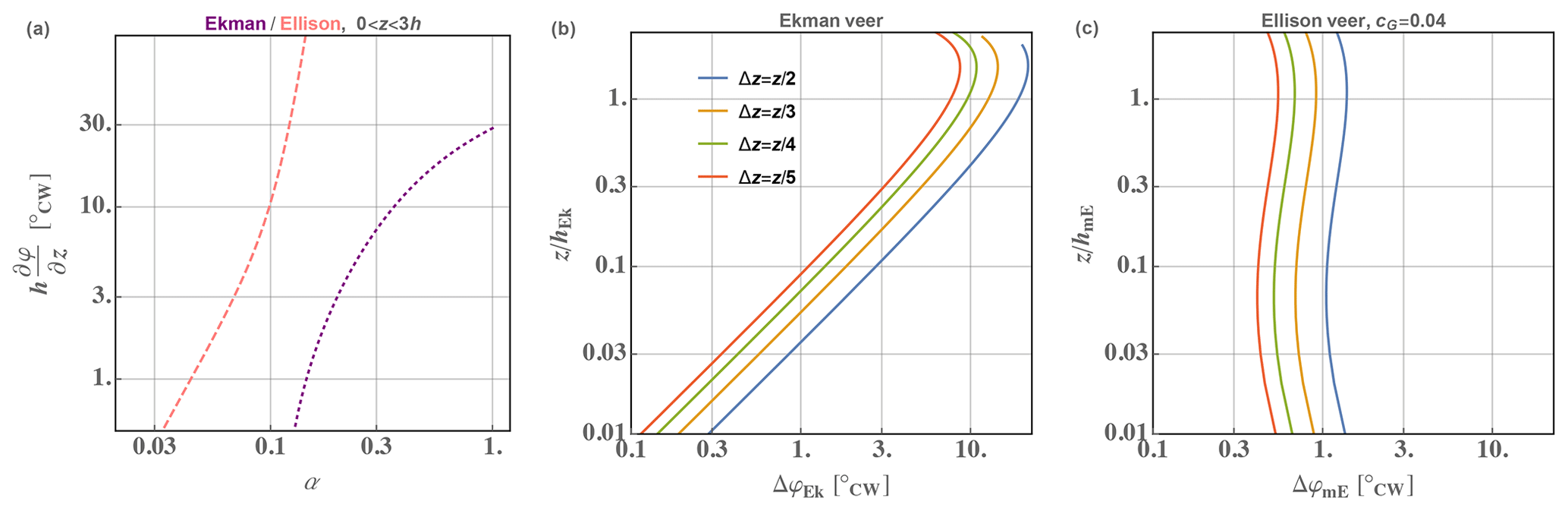
Figure 1Veer behavior (plotted as degrees clockwise) for analytical and limiting cases of Ekman and Ellison. (a) Veer versus shear exponent for any Ekman or Ellison ABL depth h; Ekman is dotted purple, and Ellison is dashed pink. (b, c) Profiles of bulk veer for different Δz; Ellison solution in (c) is the numerical solution (without approximation).
2.3.4 Ellison solution (linear diffusivity profile and surface-layer regime)
Using a surface-layer eddy-viscosity relation consistent with ASL theory, Ellison (1956) derived the solution of Eq. (7) for the (complex) wind vector, resulting in a profile of geostrophic “deficit” expressible as (Krishna, 1980)
where ker0(x) and kei0(x) are the so-called Kelvin functions (see, e.g., Abramowitz and Stegun, 1972). But the Ellison solution can be written more compactly and conveniently, similar to Eq. (24) with a complex argument, as
K0(x) is the zeroth-order modified Bessel function of the second kind, and the modified Ekman length scale is defined by , also equal to . For the range encountered in nature under neutral conditions (Hess and Garratt, 2002; van der Laan et al., 2020), for the arctangent of can be approximated via series expansions of Eqs. (28) or (29) to yield the practical result
this follows the numerical solution to within ∼20 % for , more so for cG approaching 0.04.
It was shown in van der Laan et al. (2020) that the Ekman and Ellison solutions basically gave upper and lower limits, respectively, to observed full-ABL turning (φG−φ0). Following this, in Fig. 1 we present veer profiles along with the relationship between veer and shear for the Ekman and Ellison solutions; the former is calculated via the expressions in Eqs. (25) and (27), while the latter is obtained via Eq. (29).
One can see in the left-hand plot of Fig. 1 that the Ekman solution produces effectively less mixing and consequently a higher shear exponent than Ellison's. Similarly, away from the surface (for , i.e., ) in the right-hand plots of Fig. 1 one can see the dimensionless Ekman veer exceeds that predicted by the Ellison solution; this is consistent with the Ekman ABL turning angle of ∘, which exceeds the γ0 of 5–15∘ predicted by Ellison's form (van der Laan et al., 2020). However, we note that the depth h can differ between the Ekman and Ellison solutions; hEk=hmE only if one chooses . We also point out that for larger cG (not shown in figure), near the surface () Ellison's veer grows larger than the peak value shown at z≈1.5hmE and relative to the behavior seen for cG=0.04; however, this idealized near-surface behavior is likely not relevant for wind applications.
2.4 Practical forms and application
To use the expressions derived for veer earlier, one needs the vertical derivatives of stress (or its profile) and the geostrophic wind speed; in particular the first and second vertical derivatives of the crosswind stress 〈vw〉⟂ appear in Eqs. (14) and (16), along with . In wind energy applications, engineers typically lack site-specific stress profiles unless they are taken from flow modeling; if the latter is reliable, then there is probably less need for the shear-based estimates for veer given in this work. The large-scale horizontal pressure gradients which drive ABL flow, expressible as the geostrophic wind G, are likewise rarely measured (though lidar measurements above the ABL can make this possible, e.g., Pedersen et al., 2013). The shear contribution to veer is multiplied by in Eqs. (14)–(16). To obtain a practical form relating shear to veer, we can start by parameterizing ; fortunately is commonly calculated in practice using a geostrophic drag law (GDL; Rossby and Montgomery, 1935). Long used in wind applications such as WAsP (Troen and Petersen, 1989) and related wind resource software, it is expressible in scalar form as
with components
where the empirical coefficients {A,B} are assumed to be constants in typical wind application. The geostrophic drag coefficient and ABL turning (cross-isobar angle) φG are seen to vary with surface Rossby number Ro0 (Blackadar and Tennekes, 1968); these and {A,B} have been shown to depend on dimensionless stability (Arya, 1978; Kelly and Troen, 2016), strength of ABL capping inversion (Zilitinkevich and Esau, 2002), and baroclinity (Arya and Wyngaard, 1975; Nieuwstadt, 1984). For practicality, we start by assuming near-neutral stability, which is appropriate in the mean for most places, as it represents by far the most frequently observed conditions (Kelly and Gryning, 2010); we continue to neglect baroclinity; and we neglect the influence of the capping inversion strength.9 With such assumptions, one can also write an (approximate) “reverse” form of Eq. (31) to get the drag coefficient as (Troen and Petersen, 1989)
where the surface Rossby number is and crGDL is taken to be 0.485 following its use in the wind resource program WAsP for several decades. Alternate forms of Eq. (33) exist, such as that of Hess and Garratt (2002); the latter corresponds simply to setting A=1.28 and crGDL=0.472 in Eq. (33). For a given roughness length z0 and measured wind speed , lacking the (surface) friction velocity u*, one needs a relation to connect u* and in order to get . This can be done through the same wind profile relation upon which the GDL is built, i.e., the log-law; one can use within Eq. (31) or alternately using Eq. (33), where in the latter Eq. (31) is also employed to find within Ro0.
In practice one would like a direct estimate for the veer, using the routinely measured shear, since α is seen to drive . One way could be to just ignore the stress divergence terms in Eqs. (14) or (16), which with calculation of mentioned just above considerably simplifies the problem. However, this might not be justified, particularly if is not negligible compared to , as seen from comparing contributions to Eqs. (14)–(16); this can be seen using the scaling , where h is the ABL depth (e.g., Wyngaard, 2010). Thus we consider estimating vertical derivatives of the stresses, starting with the just mentioned, which can be used in Eq. (16). Similarly, one can estimate or
where is the Rossby number based on ABL depth and of order 1; we will treat cvw as an empirical constant which is tuned later below. To use Eq. (16) we also need to find sin φG; employing Eq. (32) and using trigonometric identities to expand sin (φ−φ0), with some rearrangement one obtains
Employing this, Eq. (34), and , along with Eqs. (31) or (33), allows one to then use Eq. (16).
On the other hand, using Eq. (14) is simpler and more convenient than Eq. (16) because it only requires in addition to the second derivative of 〈vw〉 just approximated in Eq. (34) above, so one can also simply approximate and use Eq. (34); the GDL forms Eqs. (31) and (33) which then allow one to get Roh and cG, respectively. Whether using Eq. (16) or (14), we note that the shear contribution to veer includes a surface Rossby number (Ro0) dependence through , while the stress–Coriolis contribution includes an ABL-depth dependence, Roh; either way, if we do not neglect the latter, then we also need an estimate for the ABL depth h. If the shear contribution is expected to dominate variations in veer, then the estimate of h may not be so crucial; we will consider this further below in our comparison with real-world cases and also direct interested readers to, e.g., Liu and Liang (2010) for statistics of h in different conditions.
This section presents an analysis of results from RANS simulations of the neutral atmospheric boundary layer10 and of observations at different sites (which include the impacts of stability). The simulations are analyzed to check the relations given here, as well as examine the behavior of and contributions to veer across the range of Rossby numbers (Ro0 and Roh) encountered in nature. An investigation of observations, spanning turbine rotor heights for six different flow regimes and conditions across four locations, includes probing the interconnected behaviors of shear (exponent) and veer with atmospheric stability – as well as their joint statistics, universal trends, and variation with wind speed. The statistical demonstration of observations is accompanied by predictions of veer using empirically updated forms of the relations given in the previous section, as well as the forms themselves.
3.1 RANS simulations of neutral ABLs
3.1.1 Model and setup
The Navier–Stokes solver Ellipsys1D (van der Laan and Sørensen, 2017), which is a one-dimensional version of the multiblock general computational fluid dynamics (CFD) solver Ellipsys3D (Sørensen, 1995), was used to simulate the Reynolds-averaged flow in neutral atmospheric boundary layers, including Coriolis forces. Assuming zero vertical velocity and constant pressure gradients, it solves the RANS equations for incompressible flow with a finite-volume scheme. The ABL “top” (above which turbulence is extinguished) is modeled via the length-scale limiter model of Apsley and Castro (1997) implemented into the k–ε turbulence closure equations solved by Ellipsys1D, as outlined in van der Laan et al. (2020); this includes the use of small ambient values of turbulence intensity and dissipation rate above the ABL, with k–ε constants Cμ=0.03, Cε1=1.21, Cε2=1.92, σk=1.0, and σε=1.3. The k–ε model provides the stresses occurring in the RANS equations, via the flux-gradient relation and ; thus we see that such turbulence closure gives stresses aligned with velocity gradients.
The domain height is set to 105 m to ensure it is much larger than h for all simulations, and the bottom boundary is handled by a rough-wall condition (Sørensen et al., 2007). The numerical “grid” is a vertical line, with the bottom cell height being 1 cm (placed above the roughness length) and the cells' sizes growing progressively upward with an expansion ratio of 1.2; the total number of cells is 384. At the bottom cell a Neumann condition is set for k () and ε is set to the logarithmic value, and the wall stress is consequently defined by the neutral surface layer for this cell. More details, including a grid-refinement study, may be found in van der Laan et al. (2020).
Using a constant geostrophic wind speed, the flow is driven by a constant pressure gradient, starting with an initial wind profile set to at all heights; the ABL depth grows upward until convergence occurs, providing a steady solution and h for a given choice of z0, pressure gradient (thus G and f), and turbulence (k–ε) limiting length scale ℓmax. The Buckingham pi theorem can be used to reduce the four parameters into two dimensionless groups, namely Rossby numbers for z0 and ℓmax; for length-scale-limited k–ε RANS in the neutral ABL, one further has the relation (van der Laan et al., 2020)
thus giving us the two Rossby numbers Ro0 and Roh for describing flow cases (van der Laan et al., 2020). Simulations were done over the full range of ABL depths, surface roughnesses, and wind speeds encountered in nature, which correspond to a range of Rossby numbers spanning 10 and . For simplicity was set to 10 m s−1 and f to 10−4 s−1 in the simulation set spanning these ranges of Rossby numbers. However, note that Rossby similarity means that for a given pair of {Ro0,Roh} and {z0,h} one has many (infinite) combinations of which give the same and thus the same dimensionless profile shapes of velocity, i.e., speed and direction as a function of dimensionless height . At any rate, the simulations cover ranges of (exceeding) the following: ABL depths of 200–2000 m, roughness lengths from water's roughness (0.1 mm) up to 2.5 m, and from 5–50 m s−1.
3.1.2 Shear and veer over neutral ABLs simulated over entire range of Rossby numbers found in nature
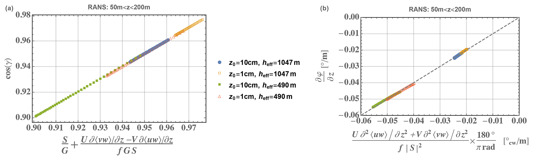
First we check that the RANS simulations confirm the shear–veer relations developed earlier; we expect this to be, since there are no extra terms in the simulated Navier–Stokes equations compared to Eq. (7). Figure 2 displays both sides of Eqs. (9) and (13) for four cases representing somewhat common real-world conditions for heights between 50–200 m.
From Fig. 2 one can see that the Ellipsys1D solutions conform to Eqs. (9) and (13) derived earlier.
Towards investigating the behavior of veer (and shear) in terms of Rossby numbers – which is facilitated by RANS but is quite difficult to accomplish with measurements – we turn our attention to the variation in veer as a function of surface roughness. Admitting that we are using one-dimensional simulations over a homogeneous surface, we now consider the directional change across typical turbine rotor heights, i.e., Δφ from z=50 to 150 m. Figure 3 displays plotted over different roughnesses for the two ABL depths represented in the cases shown in the previous figure, namely 490 and 1047 m.
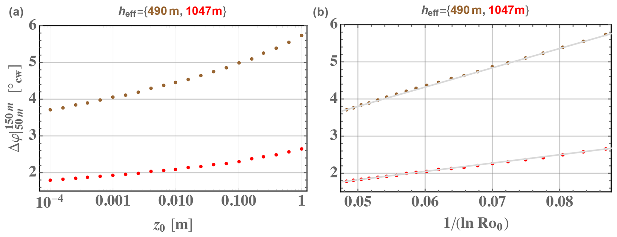
Figure 3Roughness dependence of turning (in degrees clockwise) seen for two representative ABL depths from one-dimensional RANS simulations over a range of roughness lengths plotted directly against z0 (a) and alternately versus (b). Lines in (b) indicate linear trend.
From the right-hand plot in Fig. 3 one can see that Δφ is roughly proportional to , as expected from the contribution to veer considering Eqs. (31) and (33).
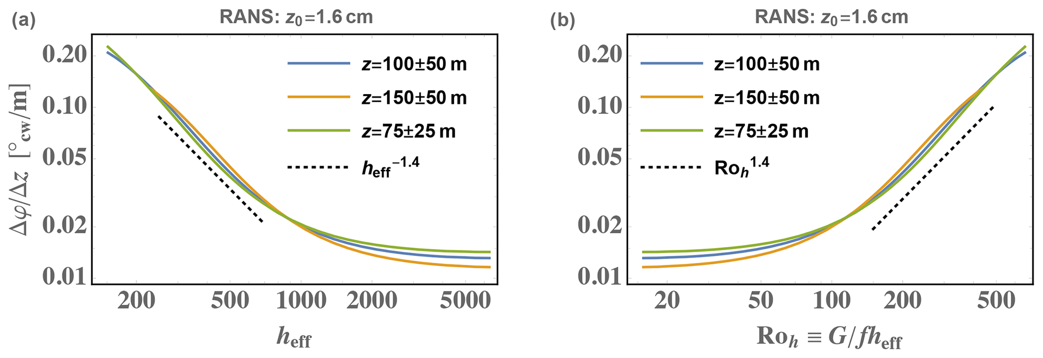
Figure 4Influence of ABL depth and associated Rossby number on veer (clockwise) for different turbine rotor spans.
Looking back on Eq. (34), we may also expect a Roh dependence in the veer, at least considering the stress gradient contributions. Figure 4 shows veer across three different rotor extents (z=50–100, 50–150, and 100–200 m), over a wide range of effective ABL depth h and associated Rossby number Roh, for a commonly found roughness over land (1.6 cm).
In Fig. 4 results are shown only for one roughness because the curves of veer versus ABL depth and Roh look nearly identical when using any other z0 (or Ro0) value, such as water roughnesses less than 0.3 mm. In other words, the sensitivity of veer to h is essentially independent of z0 if one varies these separately from case to case as in our numerical simulations. Looking at these results, we note a behavior that is consistent with the estimates for stress-gradient contributions following Eq. (34): as indicated by the dotted lines in Fig. 4, the veer is empirically found to be proportional to (or h−1.4) over a range of ABL depths routinely observed in reality (h∼200–800 m); the dependence softens to be linear in Roh (or ) for depths approaching h∼1 km, which are also commonly observed in nature (e.g., Liu and Liang, 2010). For yet deeper ABLs which are more rarely encountered, the height dependence vanishes; this can be intuitively interpreted, as becomes so small that less directional change is found for a given Δz when h is increased further. The veer and its h dependence is seen to be basically independent of height for these 50–100 m vertical spans: at the heights of interest for wind energy shown, the lines collapse onto one another. To compare with Fig. 3, multiplying the veers in Fig. 4 by Δz=100 m for the blue and gold curves, we can also see that for a realistic range of ABL depths and roughnesses, the effect of h is stronger than that of z0: across all Ro0 a variation in of only several degrees is seen, whereas across the common range of Roh a variation of more than 15∘ is shown.
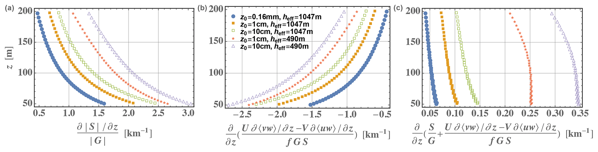
Figure 5Profiles of contributions to in Eq. (12) due to shear (a), stress gradients with Coriolis (b), and their sum (c). Five RANS simulations shown (two roughnesses and two ABL depths over land, one over sea) over typical turbine rotor heights; the listed z0 and h correspond to Rossby numbers using G=10 m s−1 and s−1.
Now that we have seen in Figs. 3 and 4 how the veer (or simply the turning Δφ for typical rotor Δz) depends on z0 and h, presumably due to the (shear) and stress-gradient contributions, respectively, it is prudent to examine the relative sizes of each of these contributions – particularly because RANS affords us this opportunity. One can cleanly separate these contributions by examining the variation in cos γ, as indicated by Eqs. (12) and (13). Accordingly, Fig. 5 presents the two contributions to the dimensionless veer derived in Eq. (12) for the four over-land cases shown in Fig. 2, as well as an over-sea case with the same ABL depth as two of the land cases.
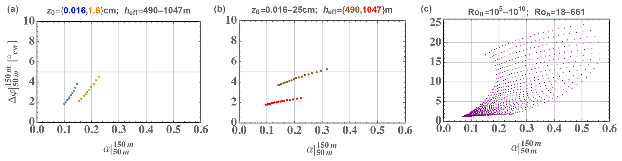
Figure 6Turning (bulk veer) in degrees clockwise versus shear exponent calculated from 50–150 m over ranges of ABL depth and surface roughness; each point represents one RANS solution. (a) Using G=10 m s−1 and s−1 over range of ABL depths spanning the values used in Figs. 2–5 for water and typical land roughness. (b) Again with G=10 m s−1 and s−1 over range of z0 spanning those used in Figs. 2–5 for two ABL (typical) depths used in previous figures. (c) Over wider range of {Ro0,Roh} spanning that found in nature; note larger vertical axis scale.
One can note from Fig. 5 that the shear and stress-gradient and Coriolis contributions largely offset each other, with each being an order of magnitude larger than their sum, which is equal to the dimensionless veer . The vertical profiles of “point-wise” veer shown in the figure, which were calculated using third-order finite difference, indicate that in neutral conditions the veer is smaller offshore compared to on land. Further, one sees the combined effect of the behaviors noted from the previous two figures: shallower ABLs have larger veer, as do ABLs over rougher surfaces, with Ro0(z0) having a smaller impact than Roh(h).
This can be put into a more practical context by considering the variation in shear and veer together across the range of Rossby numbers found in atmospheric flows. Figure 6 displays turning versus shear exponent, with each calculated across Δz from 50–150 m. The figure shows three plots of {α,Δφ}: one for a range of Roh equivalent to h ranging from 490 to 1047 m over two different z0 (land and sea), one for a range of Ro0 equivalent to z0 values varying from 0.016–25 cm for two different ABL depths h (which bracket the range of h in the left-hand plot), and one over the entire atmospheric range of both Ro0 and Roh.
From the left and center panels of Fig. 6, it becomes evident that Roh affects Δφ more than α for typical rotor extents; opposite of this, Ro0 affects the shear more than the veer. Further, for the relatively representative set of (common) cases shown in the center and left-hand plots in Fig. 6, we notice much less variation in {α,Δφ} compared to the entire parameter space displayed in the right-hand plot; as we will see in the next subsection, the right-hand plot is more in line with observations despite the RANS solutions representing nominally neutral conditions11 over uniform surfaces with neglect of shear-stress misalignment and baroclinity.
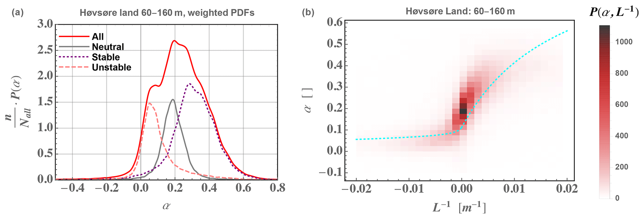
Figure 7(a) PDF of shear exponent α, weighted by frequency of occurrence for different atmospheric stability conditions; neutral is defined by m−1, stable has m−1, and unstable has m−1. (b) Joint PDF of shear exponent calculated from 60–160 m height and inverse Obukhov length (surface-layer stability) at z=10 m from sonic anemometers over the homogeneous land sectors at Høvsøre, along with M–O similarity implied by Eq. (2) shown by dashed cyan line; JPDF value of 1000 corresponds to approximately 3.5 % occurrence. Measurements span one decade, starting in 2005.
3.2 Results from measurements in different wind regimes and sites
After examining the behavior of neutral-ABL dependencies for shear and veer above from simulations, now we consider the behavior of each in the real world from measurements at different sites, which includes, e.g., the effects of stability. The datasets are the same as those analyzed by Kelly et al. (2014a), which showed shear exponent statistics for these locations, except a longer record of Høvsøre data was used for the current study (10 years, from 2005–2015). These are the aforementioned Høvsøre site, from 60–160 m height for both homogeneous land and sea sectors; the partly forested but flat Østerild site (Peña, 2019) for two virtual rotor spans, from 45–140 and 80–200 m over 1 year; the Dutch research site Cabauw (Beljaars and Bosveld, 1997), from 80–200 m height for 2 years; and 1 year from a commercial site dubbed “MR” which sits on a ridge over a mostly forested () area but dominated by hills having elevation differences up to ∼200 m within 10 km distance, using anemometers at 40–136 m height.12
We investigate the statistical behavior of veer with shear exponent as well, not only to see their interdependent behavior, but also towards providing useful relations for their variability and practical prediction of veer from typical wind energy measurement campaigns.
3.2.1 Shear exponent
Here we briefly explore the connection between probability distribution functions (PDFs) of stability and shear exponent. The shear distribution f(α) can be connected to f(L−1) in the surface layer during stable conditions, but there is not necessarily a one-to-one (unique) mapping between the two (Kelly et al., 2014a). As seen in Eqs. (4) and (5), α tends to correlate with stability () and particularly buoyant destruction (−B) during stable conditions, when turbulent transport is negligible. This is shown in Fig. 7, which displays the joint probability density of and L−1 calculated in the ASL at z=10 m from the homogeneous land sectors at the Danish national test station of Høvsøre (Peña et al., 2016) from 10 min averages over a 10-year period.
From Fig. 7 one sees the cloud of observed follow somewhat the curve of implied by M–O theory and Eq. (2) but with most α exceeding the similarity-based form; the shear exceeds M–O theory's prediction primarily due to the upper-level height (160 m) being above the surface layer.13 The left-hand panel of Fig. 7 also shows the distribution of α for neutral ( m−1), stable ( m−1), and unstable ( m−1) flow regimes, weighted by frequency of occurrence to show the relative contributions to the overall distribution. The threshold of ±0.001 m−1 for L−1 is a sensible choice because then (consistent with neutral conditions) in the surface layer, which is generally taken to have a thickness of 100 m or less (roughly , also recalling that M–O theory's applicability diminishes with height above the surface layer). Even at this relatively flat and uniform site, negative shear happens in both stable and unstable conditions, though more so in unstable and yet less often in neutral conditions; overall, α<0 occurs less than 5 % of the time over the 60–160 m span here, and 8 %–9 % from anemometers at 100–160 m heights (not shown). We also note that while the “ideal” Høvsøre land (eastern) sectors have conditions split somewhat evenly between the three stability regimes, other sites can differ (Kelly and Gryning, 2010).
3.2.2 Veer
Along with distributions of α, measured veer distributions are shown in Fig. 8 for both land and sea conditions at Høvsøre, i.e., from the homogeneous offshore/open-fetch () and over-land () directions. Shear and veer are shown calculated over height spans of 60–160 m as well as 100–160 m in the figure, which is provided to show the statistical and behavioral differences between shear and veer.
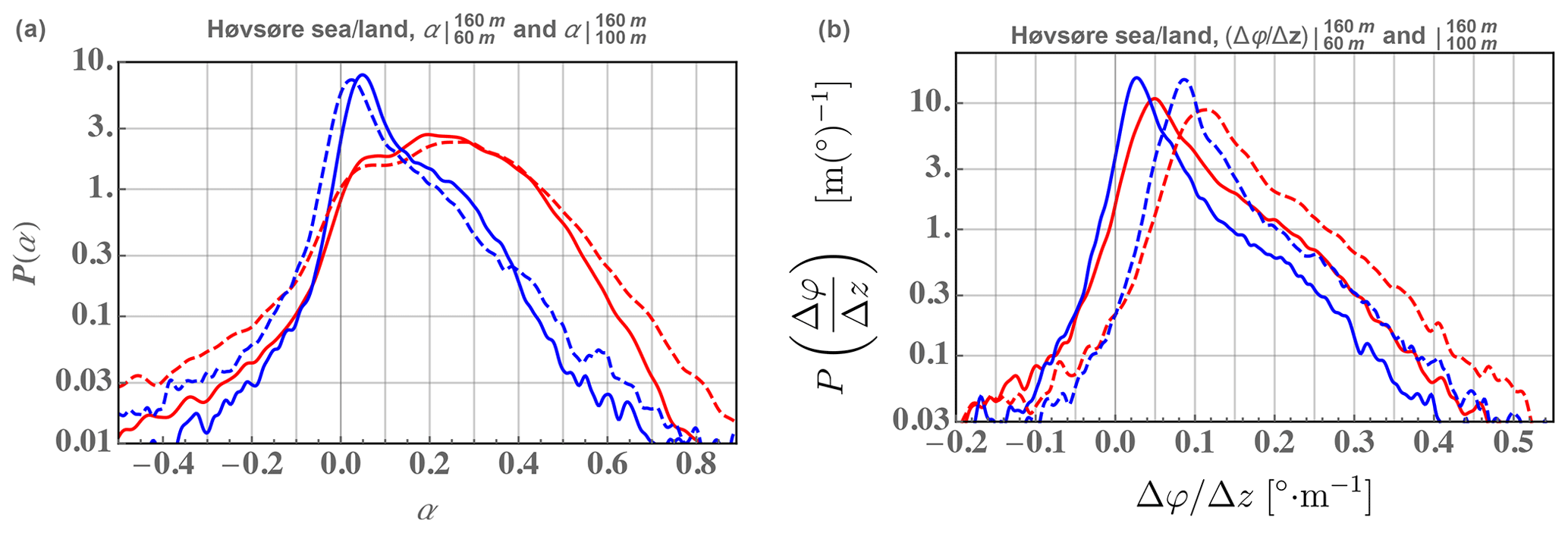
Figure 8Distributions of shear exponent (a) and corresponding veer (b) at Høvsore between 60–160 m from the homogeneous eastern land sectors (red) and from the sea sectors to the west (blue). Solid lines are for measurements spanning 60–160 m and dashed for those spanning 100–160 m.
From the two plots in Fig. 8 one can see that the most common α and , i.e., the portions of P(α) and with respective probabilities within an order of magnitude of the peak values, both systematically differ when using higher measurements at 100–160 m compared with 60–160 m heights; however, the shift in the commonest α is significantly smaller than the analogous shift in between these two height ranges. This happens over both land and sea, though both α and vary with height more for the offshore flow than for the homogeneous land directions. The change in mean shear exponent 〈α〉 from 60–160 to 100–160 m is less than +5 % over land, and % is seen over sea, while the mean veer is seen to increase by factors of and 2 over land and sea, respectively.
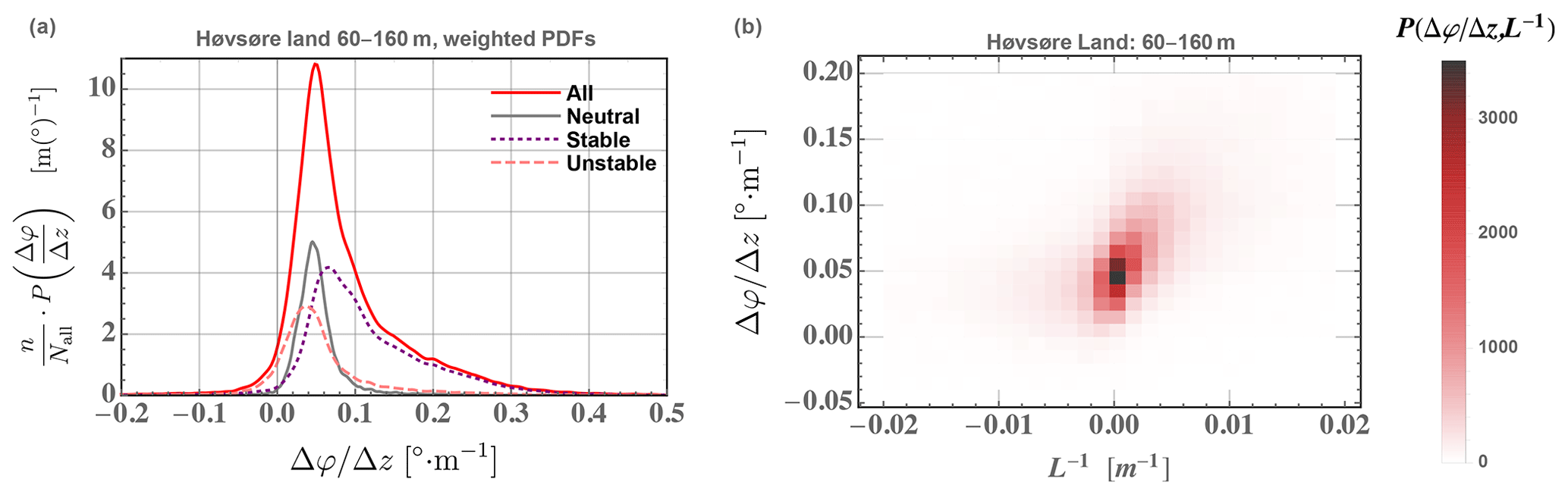
Figure 9(a) PDF of veer , weighted by frequency of occurrence for different stability conditions; neutral has m−1, stable has m−1, and unstable has m−1. (b) Joint probability distribution of veer calculated from 60–160 m height and inverse Obukhov length (surface-layer stability) at z=10 m from sonic anemometers over the homogeneous land sectors at Høvsøre; here a JPDF value of 3000 corresponds to 4.2 % occurrence. Measurements span one decade, starting in 2005.
There are several other notable differences between the shear and veer statistics shown in Fig. 8. The peak portion of P(α) is significantly wider over land compared to offshore (with larger σα over the rougher surface), while the shape around the peak does not differ significantly from land to sea here. Further, the (logarithmic) slope of versus for veer larger than the PDF peak is basically the same regardless of height or surface conditions; this and the land–sea difference between P(α) are consistent with the earlier RANS results, where z0 primarily affects α, while is impacted more by ABL depth. P(α) also has wider “tails” (extremes) higher from the ground on both sides, including negative shear due to low-level jets (such as that due to the capping inversion when h∼200 m), whereas the veer simply becomes larger due to such jets in shallow ABLs, as jets and the environment associated with the capping inversion simply cause more turning and not a reversal. The negative veer occurs due to nonstationary processes like passing fronts (e.g., Clark, 2013), as well as baroclinity and motions associated with it (Arya, 1978; Foster and Levy, 1998; Floors et al., 2015). Comparing the solid and dashed lines in Fig. 8, one sees that the highest veers are larger for the 100–160 m measurements than those from 60–160 m; this is again due to the greater impact of the ABL capping inversion and associated jet with turning.
As with shear, stability affects veer, with stable conditions expected to lead to higher veer due to its damping effect on vertical fluxes (suppressing vertical “communication” of flow information). Following the plots shown in Fig. 7 for the shear exponent α, Fig. 9 displays the effect of stability on veer for the Høvsøre land sectors. The figure shows for neutral ( m−1), stable ( m−1), and unstable ( m−1) flow regimes, weighted by frequency of occurrence (indicating relative contributions to the full PDF), as well as the joint distribution of stability and .
From Fig. 9 one sees that in comparison with P(α) shown in Fig. 7, the peaks of veer distributions do not depend so much on stability. However, as with the shear distribution, also has its largest values dominated by stable conditions; this makes sense considering that stability tends to maintain vertical gradients by limiting vertical fluxes. Unlike the results shown for the RANS simulations or predicted by theory, negative veer occurs as in Fig. 8 and is described thereunder; one can see in Fig. 9 that it basically happens during non-neutral conditions, which tend to occur at lower wind speeds, and is dominated by unstable conditions. Looking at the joint distribution one sees that for the most common veer values (∘ m−1), which tend to occur around neutral conditions, there is a mild stability dependence; however, for less neutral conditions there is little correlation between veer and stability, aside from higher veer simply being observed more often in stable conditions.
To show the behavior of veer across different locations, Fig. 10 displays the PDFs of veer from a number of sites, all of which have similar Δz and cover typical turbine rotor extents.
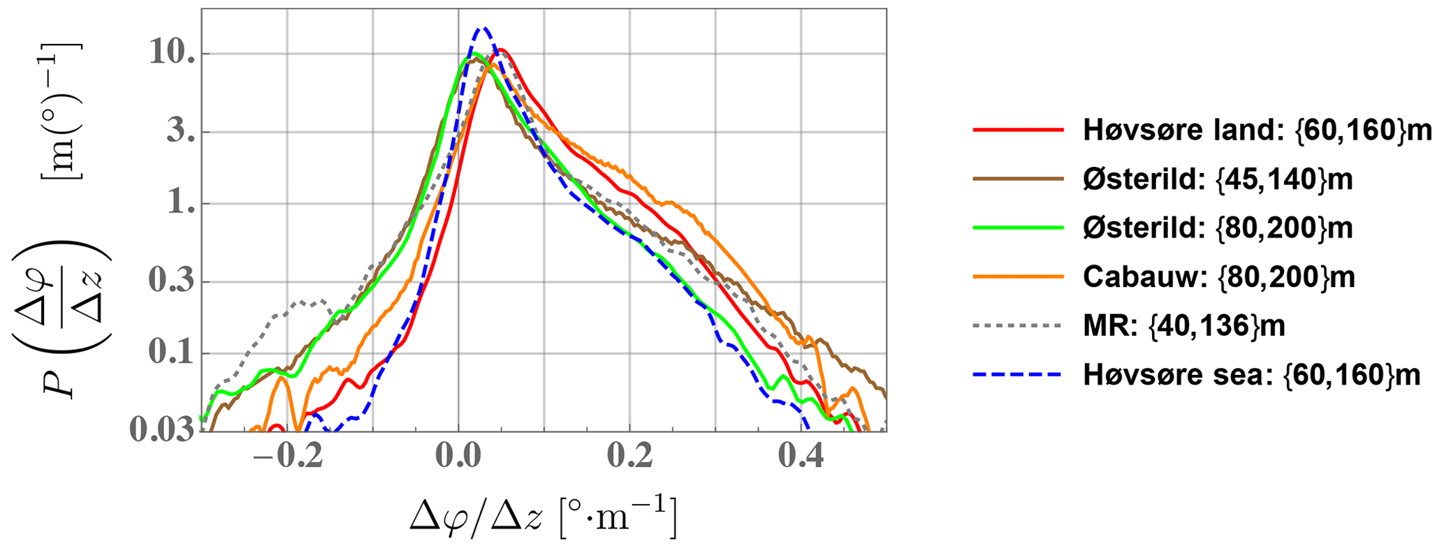
Figure 10Probability density function (distribution) of veer, , for all conditions at the various sites and cases considered.
From Fig. 10 we see that for veer magnitudes exceeding the most commonly observed values (which tend to occur in stable conditions, as shown in Fig. 9 for the Høvsøre case above), the distributions behave similarly across locations; in particular the “slope” of the semi-log plot for veer exceeding the PDF peaks is roughly constant for ∘ m−1 in each case. These slopes correspond to (conditional) PDFs for the largest veer of the form
where the characteristic veer scale defined by ranges from roughly 0.07 to 0.11∘ m−1. The lowest Υveer corresponds to the offshore Høvsøre case, while the highest Υveer matches the Østerild case from 45–140 m. We expect larger Υveer to correspond to occurrences of higher , i.e., a larger width σ+ of the stable-side distribution following Kelly and Gryning (2010); essentially the large-veer PDF in Eq. (37) is conditional on stable conditions; i.e., we could express it as . The dominance of stable conditions reported by Peña (2019) for z≳100 m at Østerild is consistent with this, though the data from z=80–200 m (green line in Fig. 10) with smaller apparent Υveer might appear to not be, considering the increasingly stable conditions higher up at this site; but looking at the Østerild curves in the figure we see that for higher veer ∘ m−1, there is consistency: the two largest Υveer values occur for z=80–200 and z=45–140 m. Future work needs to be done to explore this, since we lack air–sea temperature differences (or water–air heat flux) for the Høvsøre offshore case and stability information for the MR site, while stability effects above forests tend to be diminished and are difficult to interpret due to turbulent transport through the treetops (e.g., Sogachev and Kelly, 2016).
One also sees the peaks of in Fig. 10 are at smaller for the forest-dominated Østerild cases, with the peak of the offshore Høvsøre veer distribution falling between these and the corresponding to the land cases of Høvsøre, Cabauw, and MR. Note that the most commonly found veer values are generally dominated by neutral conditions (or modestly stable for the exceptional Østerild site above 100 m) and point out that the mode of is essentially the same (0.005–0.006∘ m−1) for the land cases that are not dominated by forest. Further considering the RANS simulation results from Fig. 6 discussed earlier, the mode of being smaller for Høvsøre offshore than for the land cases (of Høvsøre, Cabauw, and MR) can be explained by the smaller ABL depths most commonly observed offshore compared to onshore; this is consistent with the ABL depth distributions aggregated and reported by Liu and Liang (2010). The modes of found at the inhomogeneous forest-dominated site Østerild are more strongly affected by the tree-enhanced mixing (which reduces the veer magnitudes) and to a lesser extent by shallower ABLs due to the coastline 2–5 km upwind in some directions.
The dependence of veer on wind speed at the sites considered is shown in Fig. 11, which displays the joint distribution of veer and 10 min mean wind speeds, . Along with the joint distribution, the mean veer conditioned on wind speed, , is displayed.
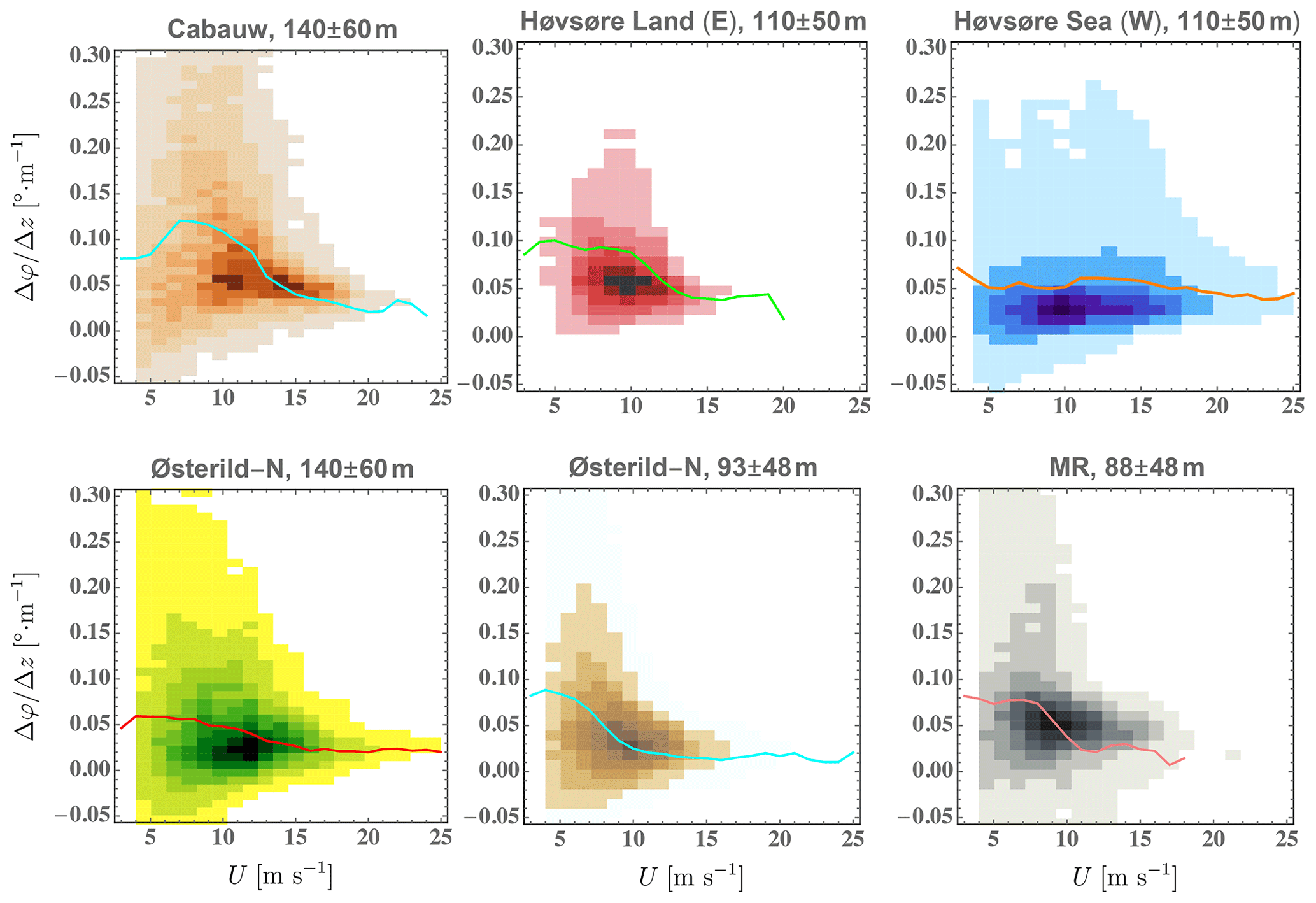
Figure 11Joint distribution of veer and wind speed at sites considered. Solid line shows , calculated using 1 m s−1 bins; lightest shades are 2 % as likely as darkest color in each plot.
From Fig. 11 one can see results consistent with the effects of stability discussed earlier and evoked by Fig. 9: at higher speeds neutral conditions dominate, giving decreased mean veer. This is more pronounced for the onshore cases (though there is still a reduction of nearly 40 % going from 12 to 24 m s−1 for the offshore case) because sea–air heat fluxes and associated magnitudes tend to be relatively smaller due to water's large heat capacity (e.g., Cronin et al., 2019). It is notable that for the representative wind turbine rotor heights considered, the veer tends to be largest for wind speeds below typical turbine rated speeds, especially over land; this can have consequences on both the power output and effective power curve for pre-construction annual energy production (AEP) estimates, as well as loads.
Further, a narrower range of veer with increasing wind speed is seen in Fig. 11, regardless of surface properties; such narrowing is impacted by stability but also occurs in neutral conditions. The variability in veer with mean wind speed is presented in Fig. 12, which displays the standard deviation of veer conditioned on mean wind speed for the sites and cases considered. It also adds a line to show the over-land Høvsøre case filtered for neutral conditions.
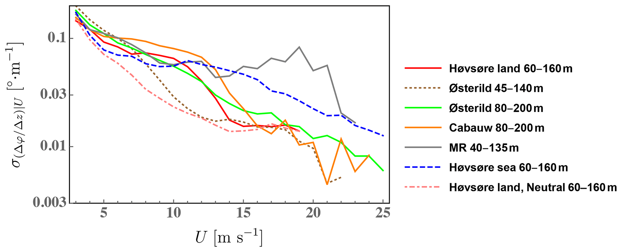
Figure 12Measured standard deviation of veer conditioned on wind speed, again using 1 m s−1 bins, for the sites considered. Neutral conditions at Høvsøre are defined as in earlier figures, i.e., m−1.
Consistent with the joint-PDFs in Fig. 11, from the semi-logarithmic plot of standard deviation of veer conditioned on mean wind speed in Fig. 12 we can see that the variation in veer decreases with wind speed and more so over land than water. It is also seen that for the onshore Høvsøre case is smaller in neutral conditions compared to over all stabilities, with the two values converging at higher speeds due to the increasingly neutral conditions. For each site having a standard deviation of veer over all speeds and mean wind speed 〈U〉, the rms veer conditioned on wind speed roughly follows the empirical form
up to about 12 m s−1 over land and to higher speeds offshore. A more complicated speed-dependent variability in veer is seen for the MR case, with higher at speeds above 15 m s−1 caused (presumably) by hill-induced turning. This has two consequences worth mentioning: firstly, that turbines at a site such as MR can experience persistent veer above rated speed, potentially increasing loads and/or reducing power below rated; and secondly, such speed-dependent behavior is likely difficult to capture with standard single RANS simulations, demanding more detailed treatment to handle the Reynolds-number dependence despite the lack of stability effects at such speeds.
3.3 Relating veer to shear in application
One of the aims of this work is to relate veer to shear (or shear exponent), as with the expressions developed in Sect. 2.3 and 2.4. Here we present joint observations of shear exponent and veer and, following these, give practical simplified forms based on the equations derived earlier in Sect. 2.3 and 2.4.
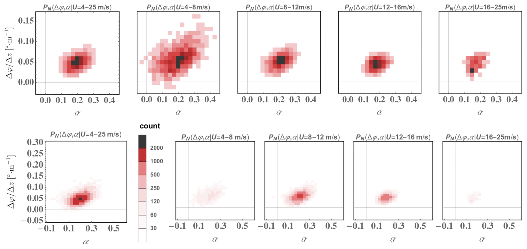
Figure 13Top panels: joint distribution of veer and shear exponent observed over 10 years from 60–160 m for the Høvsøre land sectors in neutral conditions in different speed ranges; axes zoomed in to show detail, and occurrence rate normalized per wind speed range (each plot has a different color scale, showing occurrence rate in increments of , with the lightest shade representing 10 % as likely as the darkest shade). Bottom panels: the same joint distributions shown with unscaled rate of occurrence (number of counts per bin, 2000 corresponds to about 3.9 %); axis ranges are chosen to compare with later figures.
Following the previous subsection, we first consider the joint behavior of and α with wind speed and stability for the “simple” onshore Høvsøre case having homogeneous upwind conditions. Figure 13 shows the observed joint distribution in neutral conditions, over typical turbine operation speeds (4–25 m s−1), and separately over different speed ranges (4–8, 8–12, 12–16, and 16–25 m s−1); counts are used instead of PDF per wind speed range to show relative frequencies of occurrence.
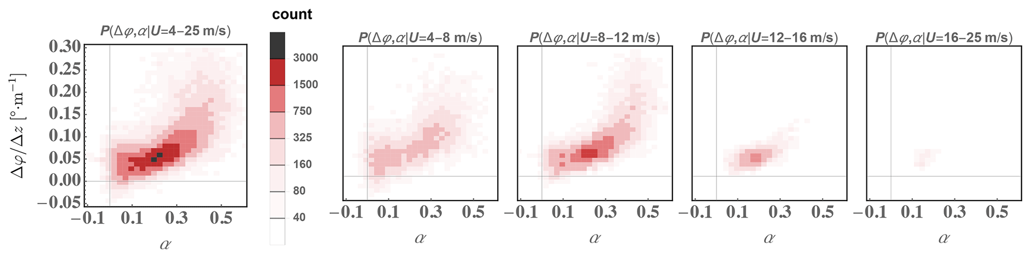
Figure 14Joint distribution of veer and shear exponent for different speed ranges from Høvsøre land sectors but for all stability conditions; plots are analogous to those in the bottom of Fig. 13. All plots use the same color scale; color bar denotes count, where 3000 corresponds to about 1.4 % occurrence.
From Fig. 13 one can notice that in neutral conditions there does not appear to be significant variation in the joint shear–veer behavior with U, with a bit more variability at the lowest speeds and smaller values of both and α for U>16 m s−1; this is consistent with Figs. 7, 9, 11, and 12. The larger spread at lower speeds for neutral conditions is attributed to the larger relative effect of nonstationarity and particularly sampling uncertainty; per the latter the integral timescale increases roughly as U−1 (Wyngaard, 2010), so fewer integral timescales are “sampled” per each 10 min period. This is also evident considering the previous plot of versus U in Fig. 12, where one sees increasing with diminishing wind speed during both neutral and all conditions for the Høvsøre land case but where stability effects cause larger veer variability up to speeds of about 15 m s−1. Also, the overall JPDF (joint PDF) appears similar to that in the most common speed range (8–12 m s−1). Aside from nonstationarity and sampling effects one does not expect much speed dependence in neutral conditions, considering the α-related part of Eqs. (14)–(16) behaves as , which following Eq. (33) has a weak dependence through ; the RANS results also confirm this. We note a joint trend between α and but also see a spread around the most common shear exponent and veer values due to variations in ABL depth, stress gradient and curvature, and top-down stability (capping inversion strength; see, e.g., Kelly et al., 2019a), in addition to nonstationarity.
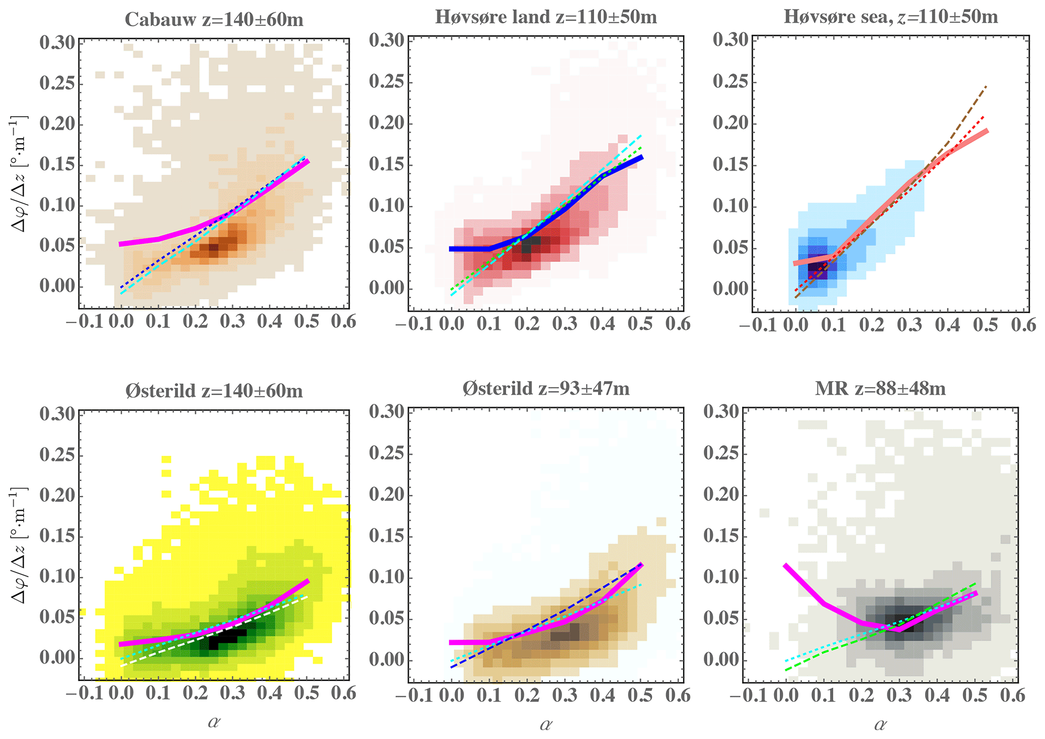
Figure 15Joint distribution P(Δφ,α) at sites considered. Solid lines: mean veer conditioned on shear exponent, ; dotted lines: simple estimate via shear portion using Eq. (39); dashed lines: estimate including estimate of crosswind stress–Coriolis contribution, Eq. (40). Lightest shades are 10 % as likely as darkest shades in each plot.
Figure 14 shows joint α-veer distributions like Fig. 13 but over all conditions, i.e., not limited to neutral stratification. One notices immediately the more frequent occurrence of higher veer and shear, as well as negative α and . Further, in addition to a wider range of shear and veer compared to neutral conditions, in Fig. 14 one can see there is also a sharper increase in with α for larger α due to stable conditions. One can see that at the most common (8–12 m s−1) and lower wind speeds, which occur in the range below rated speed for typical turbines, there is a significant increase in with α in the more stable conditions where α≳0.3; this higher “slope” of versus α is likely enhanced by the shallower ABLs which generally occur along with stable surface-layer conditions (note that the stability metric L−1 was measured in the ASL), whereby additional stable air above augments the veer. As mentioned previously, the turning and veer near the ABL top will continue to increases for yet shallower ABLs (decreasing h); meanwhile α is less sensitive to h as the upper height (used to calculate α and Δφ) exceeds the peak of the inversion-induced “jet”. Further, such high-veer conditions are not rare for such a “simple” site at the heights considered (60–160 m); e.g., conditions where and α=0.4 (a veer of 20∘ over a 100 m rotor) occur as frequently as conditions with zero shear and veer.
Towards relating veer to shear for application, we now consider the mutual behavior of Δφ and α together at all of the sites analyzed for this work. Figure 15 shows the joint distribution of shear and veer for the sites considered, with each plot also including the conditional mean of veer per shear exponent (i.e., , as solid lines).
From this figure we see a number of trends across the six cases analyzed. First, some nonlinear variation in veer with α is evident, along with the (less common) occurrence of negative values of shear and veer, as was seen in Fig. 14 for the Høvsøre land case. Further, the veer tends to be skewed towards higher values: i.e., exceeds the most commonly observed values of ; however, the MR site does not show such skewed behavior (consistent with Fig. 10), presumably due to the complex terrain there. We note the conditional mean veer is also more clearly nonlinear in α, becoming less dependent on α in low-shear (and negative) conditions; the MR site is an exception to this, with hill-induced height-dependent turning causing larger veer for α smaller than the most commonly observed values there.
3.3.1 Simplified estimate of veer per α
Figure 15 also includes two predictions based on the theory presented earlier. First, as discussed at the end of Sect. 2.4, using only the shear-associated () portion of Eq. (14) to be practical, we arrive at the estimate
compared to Eq. (14) the negative sign has been dropped to express the veer in coordinates commonly used in wind energy, i.e., clockwise positive. The basis for the simple shear-driven form can be understood by recalling Sect. 3.1 and Fig. 5, where we showed that the shear and crosswind stress-curvature contributions behaved in nearly identical but opposite fashions, with their sum amounting to ; Eq. (39) can be considered a simple model assuming the veer behaves like either of its two components but is simply smaller in magnitude. The practical form of in Eq. (39) employs the log-law for wind profile and reverse geostrophic drag law Eq. (33) for . The constant csα crudely accounts for the (competing) effects of stability on both and the geostrophic drag (and any other mechanisms affecting ) but also accounts for the smaller magnitude of compared to its shear-driven component. Within the surface Rossby number Ro0, the geostrophic speed G is calculated using Eq. (32), wherein u* is found via the log-law and with z0. To make the plots of Eq. (39) in Fig. 15 for each site, the is calculated per each bin of α, with the case-specific parameters used as well. At any rate, the practical parameterization using csα with the log-law and (neutral) reverse GDL in Eq. (39) can roughly fit the mean conditional veer at and above the most common α observed for the onshore sites considered (α≳0.2) and at α≳0.1 for the offshore Høvsøre case; here we have used effective roughness lengths consistent with earlier studies employing these sites (z0=1.5 cm for Høvsøre land, 3 cm for Cabauw, 0.9 m for Østerild, 2 m for MR, and 0.02 cm for offshore). A value of csα=0.5 can be seen to fit the heterogeneous terrain cases where terrain and roughness dominated over stability (Østerild and MR, bottom plots of Fig. 15), while for the more stability-dominated homogeneous cases (top plots in Fig. 15) a value of csα=0.7 for Høvsøre and 0.8 for Cabauw gave reasonable fits. The latter aspect could be practically addressed by directly casting csα as a minimal value plus an amount depending on the long-term variability in positive stability (labeled σ+ following Kelly and Gryning, 2010); we note Cabauw has larger values of σ+ than Høvsøre, which has larger σ+ then Østerild. However, obtaining such an expression is beyond the scope of the current article, and some sites could have factors other than stability which enhance the veer. We do find that including stability within the drag law via M–O theory (for positive L−1 values consistent with observed distributions) reduces the reverse drag-law constant by roughly 10 %–40 % for the Rossby numbers applicable at these sites, consistent with the values of csα used in the plots of Fig. 15; but again, to model stability effects beyond the surface layer becomes rather complicated and is the subject of ongoing work. For reference, a value of csα=0.6 fits the mean veer for the Høvsøre land case during neutral conditions (not shown), in contrast to the value of 0.7 which fits when all stabilities are considered there.
3.3.2 Veer estimate including both α and crosswind stress
Note that for simplicity, Eq. (39) ignored the effect of crosswind stress; it neglects not only 〈vw〉 but consequently also Roh, though it does incorporate the effect of Ro0 seen in the simulations of Sect. 3.1. Thus we also consider an approximation of the 〈vw〉 terms using Eq. (34) in Eq. (14), which introduces Roh, along with the parameterization for from Eq. (39):
where cG is found using Eq. (33), is calculated the same way as done earlier for Eq. (39), and within Roh is calculated as it was within Ro0 of Eq. (39). To use Eq. (40) the ABL depth must be prescribed, along with the constant cvw and the parameters also employed for Eq. (39). Given the negative curvature of lateral stress, (e.g., Wyngaard, 2010), cvw is negative and of order 1, with the 〈vw〉 (Roh) contribution reducing the predicted veer compared to Eq. (39). With its moderating effect on the α contribution, the 〈vw〉 part can produce an α-dependent “upturn”, though slight; this is seen for the offshore and MR cases in Fig. 15. However, the constant within is slightly larger than csα of Eq. (39) in order for Eq. (40) to fit the observed ; the values of csα=0.5 are replaced by , and csα=0.7 and 0.8 for Høvsøre and Cabauw are replaced by of 0.8 and 0.9, respectively. The value of cvw giving the estimates shown in Fig. 15 was −0.7 for all sites, while characteristic ABL depths h were taken to be 800 m over the simple land cases, 600 m offshore, and 1000 m over the hilly and forested terrain cases; we note that the results have limited sensitivity to h but choose these values to be consistent with mean ABL depth observations over sites of similar character and h distributions aggregated by Liu and Liang (2010). One can see from Fig. 15 that the estimates of using Eq. (40) are not better than the simpler form of Eq. (39), though the constants csα and cvw could easily be “tuned” together to give a better fit for each case. However, in practice one might not be able to do so and wish to simply predict veer based on α; to this end, for practical applicability we suggest using Eq. (39). Though such a recommendation would appear to be neglecting Roh and the ABL depth, we note that for estimation of mean veer (per shear) one is not so concerned with variations in Roh or Ro0 at a given site. The spread (scatter) around the mean veer seen in Fig. 15 is due to variation in stability as well as Roh or Ro0, and variation from site to site is also due to different distributions of Roh or Ro0; this is consistent with Fig. 6 and discussions following it.
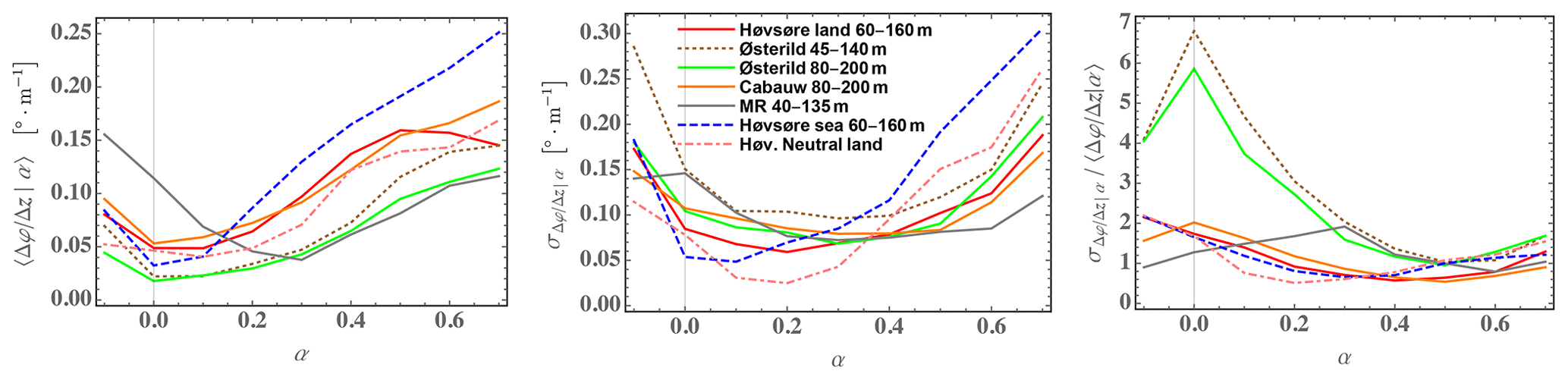
To illustrate the differences just mentioned, both the mean and standard deviation (spread) of conditional veer is shown in Fig. 16 for all the sites and cases considered.
One immediately sees the character of tends to follow the type of site; offshore has larger veer for high α, simpler sites like Cabauw and Høvsøre onshore exhibit modest veer for large α, and the more complex sites have more limited veer for α around or above its most common values of α. But note that Fig. 15 shows that high-shear conditions offshore are relatively rare and that α exceeding ∼0.3 is more common at the complex sites. We also see from Fig. 16 that for low-shear conditions (), the simpler sites exhibit higher mean veer than offshore and yet more compared to the forested cases, while much larger veer is present due to upwind hills at the MR site for such low-shear conditions (though somewhat uncommon, as seen in Fig. 15). From the middle plot we further note that the long-term variability in veer is lower offshore for the most commonly occurring α there, while veer variability does not differ so much for the most common conditions across the other sites and cases – except for the 45–140 m (lower) height range at Østerild, which shows larger veer variability due to being in the roughness sublayer above the forest there. In very high-shear conditions () the veer variability is highest offshore (though rarer). However, as shown in the right-hand plot of Fig. 16, the relative veer variability tends to more clearly show the different character of the sites: the spread of veer relative to its mean (conditioned on α) is much larger in low-shear conditions over forest, while this relative spread is similar across all non-simple (forested, complex) cases for the most commonly occurring shear; the more homogeneous sites and cases exhibit comparable under most conditions. For low-shear conditions, over more complex terrain the relative veer variability decreases, departing from the inhomogeneous forested (Østerild) values due to the large hill-induced mean veer.
The use of 〈S|α〉 in the calculations was also investigated; the plots in Figs. 15 and 16 actually incorporated mean speed conditioned on α, though use of each site's corresponding overall mean speed gave nearly identical results as those shown in the plots (within 2 %, not shown).
We have derived relationships between shear exponent (α) and veer () in a manner which avoids atmospheric-surface-layer (ASL) assumptions about meteorological parameters; this has been done in order to be applicable at wind turbine rotor heights, regardless of whether they are within or above the ASL. Canonical behavior of veer and shear with regards to surface roughness z0 and ABL depth h is also elucidated (through Rossby numbers Ro0 and Roh defined by each) through numerical solution of the one-dimensional RANS equations under neutral conditions with length-scale-limited k–ε turbulence closure (i.e., neutral but also translatable to stable conditions; see van der Laan et al., 2020).
The derived equations and RANS results essentially show that veer most simply arises from two contributions: the shear and the vertical variation in crosswind shear stress at a given height (mostly through but also via ). The numerical RANS solutions show that the shear and crosswind-stress contributions mostly offset each other in neutral conditions and that each is much larger (up to an order of magnitude) than the veer itself. It is further seen that α primarily depends upon surface roughness in neutral conditions, with a weaker dependence on ; in contrast, more strongly depends on the ABL depth h, increasing as , where n is between 1 and 1.4 for the h most commonly encountered in nature (though does also vary with ). These behaviors are consistent with the shear–veer relations derived in Sect. 2.3. We note that in this work we have also derived the cause of misalignment between shear and stress, as well as its contribution to veer; note that RANS solutions using mixing-length-type closures (as well as, e.g., Weather Research and Forecasting planetary boundary layer (WRF PBL) schemes which lack turbulent transport) give stress aligned with shear, while the analytic shear–veer relations derived here allow for misalignment through the crosswind stress.
The actual “real-world” behavior of shear exponent and veer has also been investigated from multi-year measurements at four sites covering six different flow conditions (one with separate land and offshore sectors, one with measurements both in and above the roughness sublayer over a forest) for height spans or effective rotor diameters ranging from 47–60 m centered around (hub) heights of 88–140 m. The observed include effects not fully accounted for in the equations derived here, particularly horizontal turbulent transport due to terrain inhomogeneities (Kelly, 2020) and nonstationary/transient flow conditions; though buoyancy is not explicitly accounted for, it primarily affects α and the stress, which are already incorporated into the derived veer equations.
The effect of surface-based atmospheric stability on shear and veer was examined for the relatively ideal (homogeneous) onshore site Høvsøre, where it is seen that unstable conditions dominate the low (negative) tails of the distributions P(α) and , while stable conditions are responsible for large α and ; neutral conditions contributed mostly to the peaks of the shear and veer distributions. Stability effects are consequently seen to increase the long-term variability in veer and shear, as well as veer for a given α – particularly for the commonly occurring wind speeds which tend to occur below the rated speed of modern wind turbines (e.g., Appendix B of Kelly and Jørgensen, 2017). The mean of both α and was larger compared to neutral conditions due to stably stratified conditions enhancing α and more than unstable conditions (we note that sites having a distribution of more dominated by unstable conditions, possibly some offshore, could have mean behavior similar to that found in neutral conditions).
A comparison between offshore and homogeneous onshore sectors at Høvsøre showed α to be smaller offshore (as one would expect), with more extreme values at higher z (160 m) above the surface layer regardless of the surface; the latter is presumably due to the effect of the capping inversion for ABL depths which occasionally approach such heights (Liu and Liang, 2010; Kelly et al., 2014b). The veer distributions also show larger values over land compared to offshore, though to a lesser extent than P(α); but in contrast to α, which can increase or decrease (with wider extremes) due to the position of the jet associated with the capping inversion, increases overall with z through the jet as the surface-based stress decreases with height (though there can be occasional deviations from this behavior due to stress profiles affected by upwind inhomogeneities or large coherent structures).
Two practical shear–veer relationships were derived, including parameterizations for typically unmeasured quantities contained within them, and then compared to the joint distributions and the measured from all sites over all conditions. A simplified form Eq. (39) neglecting the stress contributions was tested, as well as one Eq. (40) containing the crosswind stress. Due to the relative simplicity of the practical shear–veer forms (and additional phenomena not included in them), they needed to be calibrated in order to match observed : basically one coefficient in Eq. (39) and two in Eq. (40), all of which were of order 1 and universal (constant) across all six sites and flow situations analyzed. The form Eq. (40) for veer including crosswind stress did not give a better match to observations of across sites, compared to the simpler formula (Eq. 39), and so we recommend the latter for shear-based predictions of veer at this time. Both forms provide their best predictions (within 10 % of observed) for during the most commonly observed (moderate speeds and shear) and highest-impact (large-veer and stable) situations, with underpredictions of mean veer occurring in low-veer conditions. The observed is nonlinear in α, whereas the derived forms were nearly linear, with the inclusion of crosswind stress containing only a slight implicit nonlinearity. Lacking turbulent transport, our predictive mean veer relations are more suited for neutral and stable conditions where transport is less significant (e.g., Wyngaard, 2010); the underpredictions for smaller α, dominated by unstable conditions, evoke this. Consistent with this, the hilly MR site shows yet more low-shear deviation from our predictions due to inhomogeneity-related horizontal transport (recalling that low shear means less shear production of TKE).
Beyond the comparison of derived analytical forms with measurements of conditional mean veer , some general trends were also noted. For a given α≳0.2, was larger offshore than for the onshore cases (though note that larger α is relatively rarer offshore compared to onshore conditions); this larger mean veer for a given α is due to the ABL depth h generally being lower offshore (see, e.g., Liu and Liang, 2010, for offshore and onshore h). Perhaps counterintuitively, over the forested site the mean veer was smaller than other sites. As for the mean veer, for α≳0.3 the long-term variability was also found to be larger offshore; this may have an impact on yaw error statistics and may be the subject of future research. Analogous to σα|U found in Kelly et al. (2014a) for shear, an empirical expression for the standard deviation of veer conditioned on wind speed () was also found, with an approximately exponential decrease with speed.
Ongoing and future work
While the current work provided both theoretical meteorological relations and practical forms for veer in terms of shear, it did so without explicit treatment of buoyancy nor turbulent transport. Some relations including stability within in the shear contribution to veer were developed and tested; however, these were not included here, as they did not offer improvement, are seen to be beyond the scope of the current work, and might also require stability effects to be explicitly incorporated within the cross-stress terms. Ongoing work involves addressing the latter: i.e., self-consistent α-based description of stability within the veer formulations and within both the shear and cross-stress contributions in concert with the stability-perturbed geostrophic drag law (Arya and Wyngaard, 1975; Kelly and Troen, 2016). Future work includes the incorporation of terrain-induced turbulent transport parameterization (following e.g., Kelly, 2020) into the veer, as well as study of the latter via LES.
Because the veer at commonly occurring speeds (which occur below typical rated power) and also the mean veer are larger than for commonly assumed neutral conditions, and since we have found relations for veer variability in terms of wind speed, practical ongoing work also involves vertical extrapolation of veer and accounting for its effect on power production. Accompanying this is validation and uncertainty quantification towards pre-construction resource assessment as well as load calculations.
Some of the data are proprietary and thus are not publicly accessible. Several of the datasets are available upon request (email) to the corresponding author.
MK came up with the concept, made the mathematical derivations and analysis, and wrote the text. PvdL made the RANS simulations, checked derivations, and contributed to proofreading and editing the text.
The contact author has declared that neither of the authors has any competing interests.
Publisher's note: Copernicus Publications remains neutral with regard to jurisdictional claims in published maps and institutional affiliations.
The authors would like to acknowledge DTU Wind Energy for its internal partial support of finalizing and publishing this (old) work through its Poul la Cour fellowship. The initial core of this work was also supported by the earlier EUDP “Demonstration of a Basis for Tall Wind Turbine Design” project, number 64011-0352. Discussions about the derivations with Mads Baungaard are sincerely appreciated, as are the constructively critical reviews by Dries Allaerts and Ganesh Vijayakumar.
This research has been supported by the Energiteknologisk udviklings- og demonstrationsprogram (grant no. 64011-0352).
This paper was edited by Jennifer King and reviewed by Dries Allaerts and Ganesh Vijayakumar.
Abkar, M., Sørensen, J. N., and Porté-Agel, F.: An Analytical Model for the Effect of Vertical Wind Veer on Wind Turbine Wakes, Energies, 11, 1838, https://doi.org/10.3390/en11071838, 2018. a
Abramowitz, M. and Stegun, I. A.: Handbook of Mathematical Functions with Formulas, Graphs, and Mathematical Tables, in: 9th Edn., Dover, New York, ISBN 0-486-61272-4, 1972. a
Apsley, D. and Castro, I. P.: A limited-length-scale k–ϵ model for the neutral and stably-stratified atmospheric boundary layer, Bound.-Lay. Meteorol., 83, 75–98, 1997. a, b
Arya, S. P. S.: Comparative Effects of Stability, Baroclinity and the Scale Height Ratio on Drag Laws for the Atmospheric Boundary Layer, J. Atmos. Sci., 35, 40–46, 1978. a, b
Arya, S. P. S. and Wyngaard, J. C.: Effect of baroclinicity on wind profiles and the geostrophic drag law for the convective boundary layer, J. Atmos. Sci., 32, 767–778, 1975. a, b, c
Beljaars, A. C. M. and Bosveld, F. C.: Cabauw data for the validation of land surface parametrization schemes, J. Climate, 10, 1172–1193, 1997. a
Berg, J., Mann, J., and Patton, E. G.: Lidar-Observed Stress Vectors and Veer in the Atmospheric Boundary Layer, J. Atmos. Ocean. Tech., 30, 1961–1969, https://doi.org/10.1175/JTECH-D-12-00266.1, 2013. a, b
Blackadar, A. K.: The vertical distribution of wind and turbulent exchange in a neutral atmosphere, J. Geophys. Res., 67, 3095–3102, 1962. a
Blackadar, A. K. and Tennekes, H.: Asymptotic similarity in neutral barotrophic planetary boundary layers, J. Atmos. Sci., 25, 1015–1020, 1968. a
Bohren, C. F. and Albrecht, B. A.: Atmospheric Thermodynamics, Oxford University Press, New York, ISBN 0-19-509904-4, 1998. a
Brown, A. R., Beljaars, A. C., Hersbach, H., Hollingsworth, A., Miller, M., and Vasiljevic, D.: Wind turning across the marine atmospheric boundary layer, Q. J. Roy. Meteorol. Soc., 131, 1233–1250, https://doi.org/10.1256/qj.04.163, 2005. a
Brugger, P., Fuertes, F. C., Vahidzadeh, M., Markfort, C. D., and Porté-Agel, F.: Characterization of Wind Turbine Wakes with Nacelle-Mounted Doppler LiDARs and Model Validation in the Presence of Wind Veer, Remote Sens., 11, 2247, https://doi.org/10.3390/rs11192247, 2019. a
Businger, J. A., Wyngaard, J. C., Izumi, Y., and Bradley, E. F.: Flux-profile relationships in the atmospheric surface layer, J. Atmos. Sci., 28, 181–189, 1971. a
Carl, D. M., Tarbell, T. C., and Panofsky, H. A.: Profiles of Wind and Temperature from Towers over Homogeneous Terrain, J. Atmos. Sci., 30, 788–794, 1973. a
Choukulkar, A., Pichugina, Y., Clack, C. T., Calhoun, R., Banta, R., Brewer, A., and Hardesty, M.: A new formulation for rotor equivalent wind speed for wind resource assessment and wind power forecasting, Wind Energy, 19, 1439–1452, https://doi.org/10.1002/we.1929, 2016. a
Clack, C. T., Alexander, A., Choukulkar, A., and MacDonald, A. E.: Demonstrating the effect of vertical and directional shear for resource mapping of wind power, Wind Energy, 19, 1687–1697, https://doi.org/10.1002/we.1944, 2016. a
Clark, M. R.: Investigating cold-frontal gradients in surface parameters using operationally-available minute-resolution data, Meteorol. Appl., 20, 405–416, https://doi.org/10.1002/met.1298, 2013. a
Clarke, R. H.: Note on baroclinicity and the inverse behaviour of surface stress and wind turning in the boundary layer, Contrib. Atmos. Phys., 48, 46–50, 1975. a
Cronin, M. F., Gentemann, C. L., Edson, J., Ueki, I., Bourassa, M., Brown, S., Clayson, C. A., Fairall, C. W., Farrar, J. T., Gille, S. T., Gulev, S., Josey, S. A., Kato, S., Katsumata, M., Kent, E., Krug, M., Minnett, P. J., Parfitt, R., Pinker, R. T., Stackhouse, P. W., Swart, S., Tomita, H., Vandemark, D., Weller, A. R., Yoneyama, K., Yu, L., and Zhang, D.: Air-Sea Fluxes With a Focus on Heat and Momentum, Front. Mar. Sci., 6, 430, https://doi.org/10.3389/fmars.2019.00430, 2019. a
Derbyshire, S. H.: Nieuwstadt's stable boundary layer revisited, Q. J. Roy. Meteorol. Soc., 116, 127–158, https://doi.org/10.1002/qj.49711649106, 1990. a
Dimitrov, N., Kelly, M. C., Vignaroli, A., and Berg, J.: From wind to loads: wind turbine site-specific load estimation with surrogate models trained on high-fidelity load databases, Wind Energ. Sci., 3, 767–790, https://doi.org/10.5194/wes-3-767-2018, 2018. a
Ekman, V.: On the influence of the Earth's rotation on ocean currents, Math. Astron. Phys., 2, 1–52, 1905. a
Ellison, T. H.: Atmospheric Turbulence, in: Surveys in mechanics: A collection of surveys of the present position of research in some branches of mechanics, written in commemoration of the 70th birthday of G. I. Taylor, edited by: Batchelor, G. and Davies, R., Cambridge University Press, p. 475, 1956. a
Floors, R., Pena, A., and Gryning, S.-E.: The effect of baroclinity on the wind in the Planetary boundary layer, Q. J. Roy. Meteorol. Soc., 141, 619–30, 2015. a
Foster, R. and Levy, G.: The Contribution of Organized Roll Vortices to the Surface Wind Vector in Baroclinic Conditions, J. Atmos. Sci., 55, 1466–1472, https://doi.org/10.1175/1520-0469(1998)055<1466:TCOORV>2.0.CO;2, 1998. a
Gao, L., Li, B., and Hong, J.: Effect of wind veer on wind turbine power generation, Phys.f Fluids, 33, 015101, https://doi.org/10.1063/5.0033826, 2021. a
Geernaert, G.: Measurements of the Angle Between the Wind Vector and Wind Stress Vector in the Surface-Layer Over the North-Sea, J. Geophys. Res.-Oceans, 93, 8215–8220, https://doi.org/10.1029/JC093iC07p08215, 1988. a
Ghannam, K. and Bou-Zeid, E.: Baroclinicity and directional shear explain departures from the logarithmic wind profile, Q. J. Roy. Meteorol. Soc., 147, 443–464, https://doi.org/10.1002/qj.3927, 2021. a
Grisogono, B.: The angle of the near-surface wind-turning in weakly stable boundary layers, Q. J. Roy. Meteorol. Soc., 137, 700–708, 2011. a, b
Hatlee, S. C. and Wyngaard, J. C.: Improved Subfilter-scale Models from the HATS Field Data, J. Atmos. Sci., 64, 1694–1705, 2007. a
Hess, G. D. and Garratt, J. R.: Evaluating models of the neutral, barotropic planetary boundary layer using integral measures. Part I: Overview., Bound.-Lay. Meteorol., 104, 359–369, 2002. a, b, c
Horst, T. W.: The footprint for estimation of atmosphere-surface exchange fluxes by profile techniques, Bound.-Lay. Meteorol., 90, 171–188, 1999. a
Hoxit, L. R.: Planetary Boundary Layer Winds in Baroclinic Conditions, J. Atmos. Sci., 31, 1003–1020, 1974. a
Hulsman, P., Sucameli, C., Petrović, V., Rott, A., Gerds, A., and Kühn, M.: Turbine power loss during yaw-misaligned free field tests at different atmospheric conditions, J. Phys.: Conf. Ser., 2265, 032074, https://doi.org/10.1088/1742-6596/2265/3/032074, 2022. a
Irwin, J. S.: A theoretical variation of the wind profile power-law exponent as a function of surface roughness and stability, Atmos. Environ., 13, 191–194, 1979. a, b
Kaimal, J. and Finnigan, J. J.: Atmospheric Boundary Layer Flows, Oxford University Press, ISBN 0-9-506239-6, 1994. a, b
Kelly, M.: Estimation of local turbulence intensity via mesoscale stability and winds, with microscale shear and terrain, Tech. Rep. DTU Wind Energy E-0213, Wind Energy Dept., Risø Lab/Campus, Danish Tech. Univ. (DTU), Roskilde, Denmark, https://doi.org/10.11581/DTU.00000262, 2020. a, b
Kelly, M. and Gryning, S.-E.: Long-Term Mean Wind Profiles Based on Similarity Theory, Bound.-Lay. Meteorol., 136, 377–390, 2010. a, b, c, d, e
Kelly, M. and Jørgensen, H. E.: Statistical characterization of roughness uncertainty and impact on wind resource estimation, Wind Energ. Sci., 2, 189–209, https://doi.org/10.5194/wes-2-189-2017, 2017. a
Kelly, M. and Troen, I.: Probabilistic stability and “tall” wind profiles: theory and method for use in wind resource assessment, Wind Energy, 19, 227–241, 2016. a, b, c
Kelly, M., Larsen, G., Dimitrov, N. K., and Natarajan, A.: Probabilistic Meteorological Characterization for Turbine Loads, J. Phys.: Conf. Ser., 524, 012076, https://doi.org/10.1088/1742-6596/524/1/012076, 2014a. a, b, c, d, e, f, g, h
Kelly, M., Troen, I., and Jørgensen, H. E.: Weibull-k revisited: “tall” profiles and height variation of wind statistics, Bound.-Lay. Meteorol., 152, 107–124, 2014b. a
Kelly, M., Cersosimo, R. A., and Berg, J.: A universal wind profile for the inversion-capped neutral atmospheric boundary layer, Q. J. Roy. Meteorol. Soc., 145, 982–992, https://doi.org/10.1002/qj.3472, 2019a. a, b
Kelly, M., Kersting, G., Mazoyer, P., Yang, C., Fillols, F. H., Clark, S., and Matos, J. C.: Uncertainty in vertical extrapolation of measured wind speed via shear, Tech. Rep. DTU Wind Energy E-0195(EN), Wind Energy Dept., Risø Lab/Campus, Danish Tech. Univ. (DTU), Roskilde, Denmark, https://doi.org/10.11581/dtu.00000261, 2019b. a
Krishna, K.: The planetary-boundary-layer model of Ellison (1956) – A retrospect, Bound.-Lay. Meteorol., 19, 293–301, 1980. a
Li, D.: The O'KEYPS Equation and 60 Years Beyond, Bound.-Lay. Meteorol., 179, 19–42, https://doi.org/10.1007/s10546-020-00585-y, 2021. a
Lindvall, J. and Svensson, G.: Wind turning in the atmospheric boundary layer over land, Q. J. Roy. Meteorol. Soc., 145, 3074–3088, https://doi.org/10.1002/qj.3605, 2019. a
Liu, L., Gadde, S. N., and Stevens, R. J.: Geostrophic drag law for conventionally neutral atmospheric boundary layers revisited, Q. J. Roy. Meteorol. Soc., 147, 847–857, https://doi.org/10.1002/qj.3949, 2021. a
Liu, S. and Liang, X.-Z.: Observed Diurnal Cycle Climatology of Planetary Boundary Layer Height, J. Climate, 23, 5790–5809, 2010. a, b, c, d, e, f
Markowski, P. and Richardson, Y.: On the Classification of Vertical Wind Shear as Directional Shear versus Speed Shear, Weather Forecast., 21, 242–247, 2006. a
Mikhail, A.: Height extrapolation of wind data, Solar Energ. Eng., 107, 10–14, 1985. a
Moeng, C.-H. and Wyngaard, J. C.: Evaluation of Turbulent Transport and Dissipation Closures in Second-Order Modeling, J. Atmos. Sci., 46, 2311–2330, 1989. a
Monin, A. S. and Obukhov, A. M.: Basic laws of turbulent mixing in the surface layer of the atmosphere (translated by John Miller, 1959), Tr. Akad. Nauk. SSSR Geofiz. Inst., 24, 163–187, 1954. a, b
Murphy, P., Lundquist, J. K., and Fleming, P.: How wind speed shear and directional veer affect the power production of a megawatt-scale operational wind turbine, Wind Energ. Sci., 5, 1169–1190, https://doi.org/10.5194/wes-5-1169-2020, 2020. a
Narasimhan, G., Gayme, D. F., and Meneveau, C.: Effects of wind veer on a yawed wind turbine wake in atmospheric boundary layer flow, ARXIV [preprint], https://doi.org/10.48550/ARXIV.2210.09525, 2022. a
Nieuwstadt, F. T. M.: The Turbulent Structure of the Stable, Nocturnal Boundary Layer, J. Atmos. Sci. 41, 2202–2216, 1984. a
Panofsky, H. and Dutton, J.: Atmospheric Turbulence, Wiley, ISBN 978-0-471-05714-7, 1984. a
Pedersen, J. G., Kelly, M., and Gryning, S.-E.: The effect of unsteady and baroclinic forcing on predicted wind profiles in Large Eddy Simulations: Two case studies of the daytime atmospheric boundary layer, Meteorol. Z., 22, 661–674, 2013. a, b
Peña, A.: Østerild: A natural laboratory for atmospheric turbulence, J. Renew. Sustain. Energ., 11, 063302, https://doi.org/10.1063/1.5121486, 2019. a, b
Peña, A., Floors, R. R., Sathe, A., Gryning, S.-E., Wagner, R., Courtney, M., Larsén, X. G., Hahmann, A. N., and Hasager, C. B.: Ten Years of Boundary-Layer and Wind-Power Meteorology at Høvsøre, Denmark, Bound.-Lay. Meteorol., 158, 1–26, https://doi.org/10.1007/s10546-015-0079-8, 2016. a
Petersen, E. L., Mortensen, N. G., Landberg, L., Højstrup, J., and Frank, H. P.: Wind power meteorology. Part II: siting and models, Wind Energy, 15, 55–72, 1998. a, b
Pope, S. B.: Turbulent Flows, Cambridge University Press, ISBN 978-0-521-59886-6, 2000. a
Robertson, A. N., Shaler, K., Sethuraman, L., and Jonkman, J.: Sensitivity analysis of the effect of wind characteristics and turbine properties on wind turbine loads, Wind Energ. Sci., 4, 479–513, https://doi.org/10.5194/wes-4-479-2019, 2019. a
Rossby, C. G. and Montgomery, R. B.: The Layer of Frictional Influence in Wind and Ocean Currents, Pap. Phys. Oceanogr. Meteorol., 3, 1–101, 1935. a
Rotta, J.: Statistical theory of non-homogeneous turbulence (“Statistiche Theorie nichthomogener Turbulenz”), Z. Physik, 129, 547–572, 1951. a
Santos, P., Peña, A., and Mann, J.: Departure from Flux-Gradient Relation in the Planetary Boundary Layer, Atmosphere, 12, 672, https://doi.org/10.3390/atmos12060672, 2021. a
Shu, Z., Li, Q., He, Y., and Chan, P. W.: Investigation of marine wind veer characteristics using wind lidar measurements, Atmosphere, 11, 1178, https://doi.org/10.3390/atmos11111178, 2020. a
Sogachev, A. and Kelly, M.: On Displacement Height, from Classical to Practical Formulation: Stress, Turbulent Transport and Vorticity Considerations, Bound.-Lay. Meteorol., 158, 361–381, https://doi.org/10.1007/s10546-015-0093-x, 2016. a
Sørensen, N. N.: General Purpose Flow Solver Applied to Flow over Hills, PhD thesis Risø-R-864(EN), Risø National Laboratory, Roskilde, Denmark, ISBN 87-550-2079-8, 1995. a
Sørensen, N. N., Bechmann, A., Johansen, J., Myllerup, L., Botha, P., Vinther, S., and Nielsen, B.: Identification of severe wind conditions using a Reynolds-averaged Navier-Stokes solver, J. Phys.: Conf. Ser., 75, 012053, https://doi.org/10.1088/1742-6596/75/1/012053, 2007. a
Svensson, G. and Holtslag, A. A. M.: Analysis of Model Results for the Turning of the Wind and Related Momentum Fluxes in the Stable Boundary Layer, Bound.-Lay. Meteorol., 132, 261–277, 2009. a
Triviño, C.: Validation of Vertical Wind Shear Methods, Zenodo [presentation], https://doi.org/10.5281/zenodo.5549897, 2017. a
Troen, I. and Petersen, E. L.: European Wind Atlas, Risø National Laboratory, Roskilde, Denmark, ISBN 87-550-1482-8, 1989. a, b
van der Laan, M. P. and Sørensen, N. N.: A 1D version of EllipSys, Technical Report DTU Wind Energy E-0141 (EN), Danish Technical University, Roskilde, Denmark, ISBN 978-87-93549-08-1, 2017. a
van der Laan, M. P., Kelly, M., Floors, R., and Peña, A.: Rossby number similarity of an atmospheric RANS model using limited-length-scale turbulence closures extended to unstable stratification, Wind Energ. Sci., 5, 355–374, https://doi.org/10.5194/wes-5-355-2020, 2020. a, b, c, d, e, f, g, h, i, j, k, l, m, n
Wyngaard, J. C.: Toward numerical modeling in the `Terra Incognita', J. Atmos. Sci., 61, 1816–1826, 2004. a
Wyngaard, J. C.: Turbulence in the Atmosphere, Cambridge University Press, ISBN 978-0-521-88769-4, 2010. a, b, c, d, e, f, g, h, i
Zilitinkevich, S. S. and Esau, I. N.: On integral measures of the neutral barotrophic planetary boundary layer, Bound.-Lay. Meteorol., 104, 371–379, 2002. a
Zilitinkevich, S. S. and Esau, I. N.: Resistance and heat-transfer laws for stable and neutral planetary boundary layers: old theory advanced and re-evaluated, Q. J. Roy. Meteorol. Soc., 131, 1863–1892, 2005. a
The full derivative () is used in Eq. (2) due to the horizontal homogeneity assumed by Monin–Obukhov similarity theory, from which Φm arises.
The “constant-flux layer” in surface-layer theory does not require exactly constant fluxes with height, as is often presumed. The label and assumption are that the nondimensional fluxes, normalized by ABL scales, are constant with z (Horst, 1999; Wyngaard, 2010); i.e., the ASL is the layer over which the decrease in is small compared to , roughly the bottom 10 % of the ABL.
We note that Kelly and Gryning (2010) adapted M–O theory to long-term means and Kelly and Troen (2016) extended this beyond the surface layer within the European Wind Atlas (WAsP) framework, thus addressing the stationarity and surface homogeneity aspects. However, the purpose and scope of the current article is to examine the commonly used shear exponent and its connection with veer and not on vertical extrapolation methods per se. This motivates use of α in applications such as wind energy, as Eq. (1) does not directly rely on surface-layer assumptions.
The turning angle can also be expressed in complex notation, recalling that the angle between vectors written in complex notation (here U→S and G→G) can be recovered by taking ℜ{G*S}, i.e., .
The ABL turning angle γ0 cannot exceed 45∘, according to the Ekman equations (or their numerical solution, as in van der Laan et al., 2020). However, in some situations, which tend to involve horizontal inhomogeneities, γ0>45∘, these include, e.g., baroclinity, terrain-induced turning (especially with stability), convective cells, and various persistent storm structures.
In the Southern Hemisphere, the signs are reversed: geostrophic flow around a local low in pressure moves clockwise, with surface-induced turbulence (“friction”) causing the flow to again increasingly turn towards low pressure as the surface is approached and thus γ<0.
The exception to this is if one considers heights within ∼10 %–20 % of the ABL top (e.g., Kelly et al., 2019a).
The approximation is found by series expansion in of about 0; the same result is obtainable by taking the vertical derivative of Eq. (6), i.e., .
We note Zilitinkevich and Esau (2005) gave a form for the GDL incorporating all three of these effects, and Liu et al. (2021) practically simplified that form, using large-eddy simulations (LESs) to find its empirical constants in the case of a nonzero effect of capping inversion strength per Coriolis parameter. However, the extra parameters needed are additional to what is required for the current theory given for climatological mean conditions and well beyond what is measured in practice.
The neutral RANS simulations can also be translated into equivalent stable cases within the k–ε–ℓmax turbulence closure framework of Apsley and Castro (1997), following van der Laan et al. (2020).
One could argue that our RANS solutions can also be interpreted to include stable conditions, since the length-scale-limited k–ε turbulence model can have its maximum mixing length ℓmax rewritten using the Blackadar (1962) mixing-length formulation such that plus a stability contribution, as shown in van der Laan et al. (2020). However, such an interpretation employs M–O theory along with the Blackadar-type form to “combine” a surface-layer scale ℓASL∝z with ℓmax; here we choose to keep our analysis as general as possible – avoiding particular ASL forms or assumptions, as well as models for turbulence length scale.
The details and location of the MR site cannot be shared publicly due to their proprietary nature (see also Kelly et al., 2014a). The site is located near the border between New York state (USA) and Canada, in a moderately hilly region.
The measurement height of 160 m also occasionally falls within 10 %–20 % of the ABL depth, whereby the capping inversion causes enhanced stability; to a lesser extent larger shear is also caused by minor inhomogeneities 3–7 km upwind, within a narrow range of directions.