One-to-one aeroservoelastic validation of operational loads and performance of a 2.8 MW wind turbine model in OpenFAST

This article presents a validation study of the popular aeroservoelastic code suite OpenFAST leveraging weeks of measurements obtained during normal operation of a 2.8 MW land-based wind turbine. Measured wind conditions were used to generate one-to-one turbulent flow fields (i.e., comparing simulation to measurement in 10 min increments, or bins) through unconstrained and constrained assimilation methods using the kinematic turbulence generators TurbSim and PyConTurb. A total of 253 bins of 10 min of normal turbine operation were selected for analysis, and a statistical comparison in terms of performance and loads is presented. We show that successful validation of the model was not strongly dependent on the type of inflow assimilation method used for mean quantities of interest, which had median modeling errors per wind-speed interval generally within 5 %–10 % of the measurement. The type of inflow assimilation method did have a larger effect on the fatigue predictions for blade-root flapwise and tower-base fore–aft quantities, which surprisingly saw larger errors from the assumed higher-fidelity assimilation methods. Avenues for further work are discussed and include possible improvements to the aerodynamic, structural, and controller modeling that may offer insight on the origin of the up to ∼ 40 % median overprediction of fatigue for these quantities.

1 Introduction

Aeroservoelastic turbine models based on blade element momentum theory (BEMT) and equivalent beam models remain at the center of design and certification processes for wind turbines thanks to the balance they strike between accuracy and computational efficiency (Van Kuik et al., 2016). The multiphysics tool, OpenFAST (Jonkman and Sprague, 2021), which is actively developed at the National Renewable Energy Laboratory, is one of these models. Over the years, OpenFAST has been subject to several rounds of verification against other aeroservoelastic solvers (Rinker et al., 2020) and validation against measurement (Guntur et al., 2017; Schepers et al., 2021; Asmuth et al., 2022; Boorsma et al., 2023), but changes in modern wind turbines, namely, the increased rotor size and concomitant changes in blade flexibility, blade aerodynamics, and atmospheric forcing, suggest an ongoing need to validate OpenFAST at scales relevant to industry. Importantly, this validation should be accomplished with suitable assimilation of measured inflow into the simulation environment to obtain a synthetic wind field that matches as closely as possible the inflow experienced by the turbine.

So far, validation of OpenFAST relative to full-scale measurements has adopted either (1) non-turbulent and uniform inflow (Schepers et al., 2021; Boorsma et al., 2023); (2) purely stochastic turbulent inflow (i.e., based on the spectral magnitudes of a reference flow but with random phases) that matches time-averaged statistics of hub-height wind speed, hub-height turbulence intensity, and shear profile (Schepers et al., 2021); (3) time-resolved inflow at a single point in the domain (i.e., with more distant points reverting to random phases) that matches time-averaged statistics of hub-height wind speed, hub-height turbulence intensity, and shear profile (Guntur et al., 2017); or (4) time-resolved inflow at multiple points in the domain (Asmuth et al., 2022). The strategy of combining one or more time series with a stochastic turbulence generation method as in (3) and (4) represents a compromise between the simpler approach of (2) that constrains the generated inflow only in terms of time-averaged statistics and emerging higher-fidelity approaches that combine large-eddy simulations with machine learning (Rybchuk et al., 2023). This paper adopts the second through fourth approaches, allowing comparison of the code predictions across different levels of inflow assimilation methods.

Recent efforts on other code suites have also compared across different levels of inflow assimilation methods. The data assimilation techniques considered by Pedersen et al. (2019) leveraged data from an upstream meteorological tower and included both unconstrained and constrained turbulence assimilation approaches. Surprisingly, the constrained turbulence approach increased the mean simulation errors by several percentage points for all damage equivalent loads (DELs) considered, and they attributed this to possibly unmet assumptions about frozen turbulence and about the measured flow field passing completely through the rotor disk. However, the constrained approach did outperform the unconstrained approach when considering inflow data measured from a Pitot probe mounted on one of the blades. Nybø et al. (2021) used data from a meteorological tower as the input to a simulation study on the differences of tower-bottom fore–aft and blade-root flapwise DELs between unconstrained and constrained approaches. They found that the unconstrained approach produced 27 % and 12 % underprediction of the tower-bottom fore–aft and blade-root flapwise DELs, respectively, compared to the constrained approach. Rather than using a meteorological tower or an on-blade sensor, Rinker (2022) constrained the turbulence fields to data generated from a turbine-mounted virtual lidar that sampled a simulated flow field. The constraining process produced a clear improvement of mean absolute errors for several quantities of interest (QoIs) versus unconstrained results. DEL predictions for the tower-base fore–aft bending moment improved when the constraint points from the lidar extended to at least 40 % of the rotor span from the axis of rotation.

Similar to the above three studies but considering instead the OpenFAST code suite, the objective of this current effort is to assess the value of existing inflow assimilation tools of different levels of fidelity (i.e., including both unconstrained and constrained turbulence assimilation methods) for validation of simulations of megawatt-scale wind turbine performance and loads. In addition to performing such a comparison across three levels of fidelity for the first time with OpenFAST, we here consider other validation quantities (i.e., damage equivalent loads) not included in the previous, recent studies involving OpenFAST that employed one of the four inflow assimilation approaches listed previously (Guntur et al., 2017; Schepers et al., 2021; Asmuth et al., 2022; Boorsma et al., 2023). In our work, quantitative comparison between measured and simulated turbine signals is calculated for 10 min statistics of these QoIs:

• rotor speed;

• blade pitch;

• electrical power;

• flapwise and edgewise blade-root bending moments;

• fore–aft tower-base bending moment.

The approach is an end-to-end validation, meaning that the accuracy of the inflow modeling, turbine aeroelastic modeling, and controller modeling is collectively evaluated according to the final turbine QoIs above. For the inflow modeling, we evaluate the relative merits of the several inflow assimilation methods with varying levels of simplifying assumptions as described above. For the turbine aeroelastic and controller modeling, a significant amount of attention was devoted to matching the behavior of the field turbine by incorporating proprietary information about the characteristics of the turbine and controller as closely as possible into the sub-modules of OpenFAST.

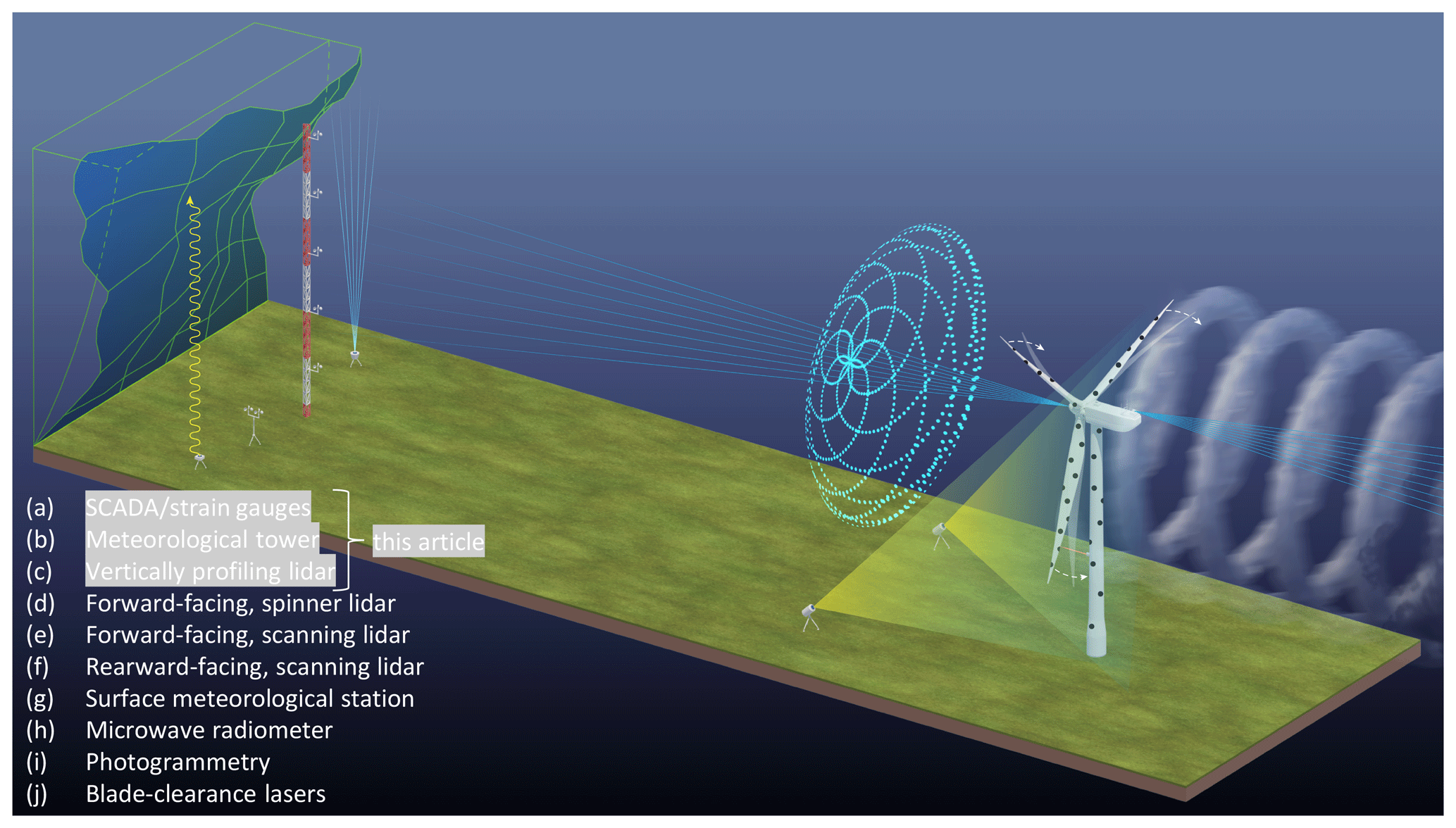
Figure 1 Illustration of the prototype wind turbine and surrounding instrumentation during the RAAW project.

The study is part of the Rotor Aerodynamics, Aeroelastics, and Wake (RAAW) experiment, which is a collaboration between the National Renewable Energy Laboratory, Sandia National Laboratories, and the wind turbine manufacturer GE Vernova. This experimental campaign leveraged a suite of measurements on a test turbine and its environment as shown in Fig. 1. The validation of the OpenFAST model presented here is based on measurements collected prior to the RAAW field campaign and is intended to benchmark the model performance. The inflow and wind turbine measurements are therefore limited to instrumentation already present at the site before RAAW as indicated in the figure.

The rest of the paper is organized as follows: the development of the turbine aeroservoelastic model is described in Sect. 2. Section 3 gives an overview of the methods for assimilation and modeling of the measured inflow data. Section 4 shows the results and is followed by suggestions for future experiments in Sect. 5. Conclusions are drawn in Sect. 6.

2 Turbine model development

The wind turbine used within the RAAW experiment is a highly instrumented 2.8 MW prototype wind turbine that mounts a rotor of 127 m diameter at a hub height of 120 m. The turbine is located in Lubbock, Texas, in a region characterized by flat terrain. More details on the instrumentation and sampling in and around the wind turbine are given in Sect. 3. The first step of this study consisted of building the OpenFAST model of the turbine. This step was performed by combining different data sets shared by GE describing the aerodynamic and elastic properties of the rotor, the elastic properties of the rest of the turbine system, and high-level information about the controller. Additionally, the GE team shared experimental results from the structural testing of the blade and numerical results from its in-house solvers. All this information was used to develop an accurate OpenFAST model. GE's proprietary controller was replaced by the publicly available Reference OpenSource Controller (ROSCO) (Abbas et al., 2022), which was tuned to the reference information and turbine sensor data. The next sections elaborate on the process used to develop this model and on the verification and validation steps that were performed.

2.1 Aerodynamics

OpenFAST can simulate rotor aerodynamics at different levels of fidelity with models implemented in the module AeroDyn15. This study models rotor aerodynamics using BEMT. The blade aerodynamic shape was discretized into 78 sections equally spaced along the blade span. A set of two-dimensional (2D) airfoil data blending clean and rough polars from wind tunnel measurements with a weighted average was shared by GE. The 2D polars were first interpolated adopting a piecewise cubic hermite interpolating polynomial scheme to match the spanwise distribution of thickness-to-chord ratio. Next, the polars of airfoils with thickness-to-chord ratios smaller than 0.7 were corrected to account for rotational effects adopting the Du–Selig model (Du and Selig, 1998). Note that the Du–Selig model relies on the successful identification of a linear regime of the lift curve, which is not obvious for airfoils located close to the blade root. This led to some arbitrary decisions about the range of angles of attack over which to apply the correction and to the decision of limiting the corrections to airfoils up to 0.7 of thickness-to-chord ratio. The airfoil unsteady behavior was modeled using an extension of the Beddoes–Leishman model developed by Minnema/Pierce (Damiani and Hayman, 2019). The parameters required by the unsteady airfoil aerodynamic model at each blade spanwise station were provided to OpenFAST as precomputed inputs.

A dynamic BEMT model that implements a continuous-time state-space form of Oye's dynamic model was used (Branlard et al., 2022). Also, the Glauert skewed wake correction model was used with a flow expansion function of $\mathrm{15}/\mathrm{32}\mathit{\pi }$ (Pitt and Peters, 1980). Other corrections to the BEMT model included the Prandtl hub- and tip-loss models, wake swirl (tangential induction), and the influence of drag on the induction factors. The effect of the tower on the incoming wind was accounted for using OpenFAST's baseline potential flow model for two of the three inflow assimilation methods as discussed further below, and tower aerodynamic loading was calculated for these two methods as well. The downstream tower shadow was not included in the modeling. The environmental conditions (i.e., inflow density and velocity) were set on a bin-by-bin basis using the data from the met tower (see Sect. 3).

2.2 Structural dynamics

The elastic response of the turbine was modeled by combining the reduced-order ElastoDyn beam model for the tower and the higher-fidelity BeamDyn model, which implements the geometrically exact beam theory (Jelenić and Crisfield, 1999; Wang et al., 2017) for the blades. The elastic properties for all turbine components were precomputed and shared by GE. The next subsections elaborate on the verification and validation steps that were performed to ensure the accuracy of the elastic model.

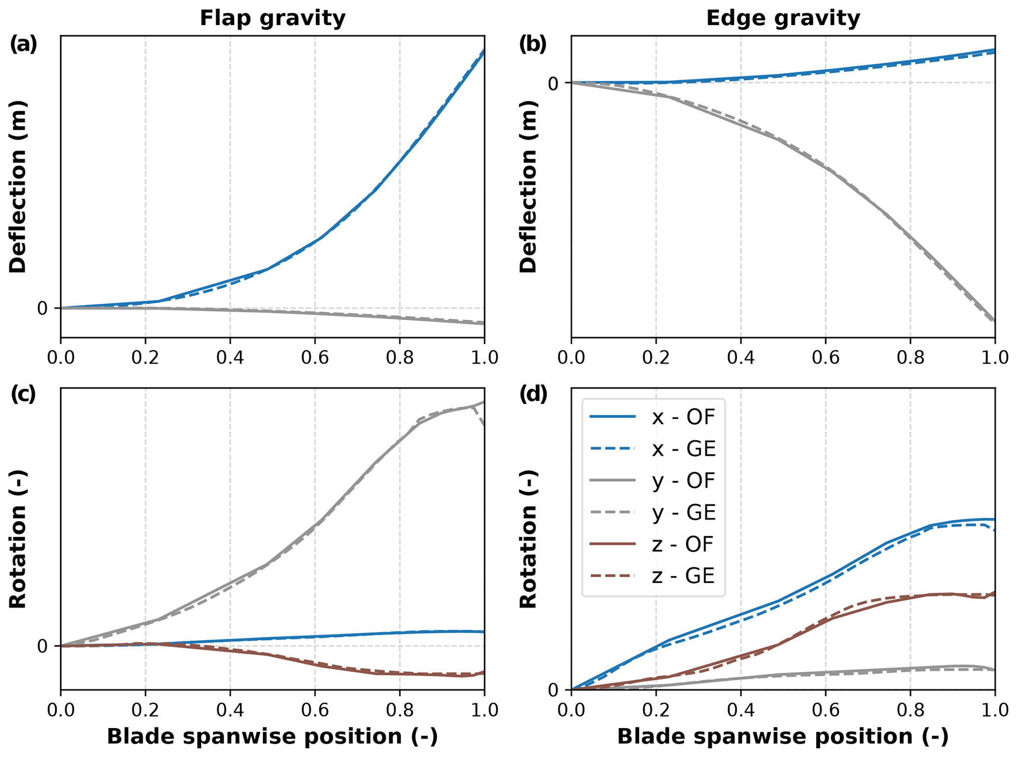
Figure 2 Deflection (a, b) and rotation (c, d) profiles of the blade loaded under gravity in the flapwise (a, c) and edgewise (b, d) directions. The dashed lines were generated by GE, and the solid lines were generated with BeamDyn, the beam model of OpenFAST implementing the geometrically exact beam theory. Results are expressed in the BeamDyn coordinate system, and rotations are expressed in terms of Wiener–Milenkovic parameters relative to the undeflected beam orientation.

2.2.1 Elastic response of the blades

GE shared detailed elastic properties of the blades. An initial verification step was then performed to confirm that the data were converted to the BeamDyn coordinate system correctly. Figure 2 shows the static deflections and rotations for a single blade clamped at the root and subjected to gravitational loads in flapwise and edgewise directions. This verification step returned maximum differences of 0.02 m in deflections and 0.5° in rotations and was considered satisfactory.

Next, a verification and validation step was performed by comparing numerical and experimental values of natural frequencies and values of structural damping for a single blade. The experimental values were generated during testing of the blade in a structural laboratory. Table 1 presents the percentage error of the blade natural frequencies and damping between the laboratory test and the numerical predictions generated at GE and in OpenFAST. The match was again satisfactory, although some important discrepancies emerged, as described next.

Table 1 Comparison of blade natural frequencies and structural damping ratios between OpenFAST and reference data including experimental and numerical values shared by GE. The values provided are in terms of percent difference relative to the experimental (“Exp”) and numerical (“Num”) reference. Positive values represent higher frequencies and damping in OpenFAST relative to the values shared by GE.

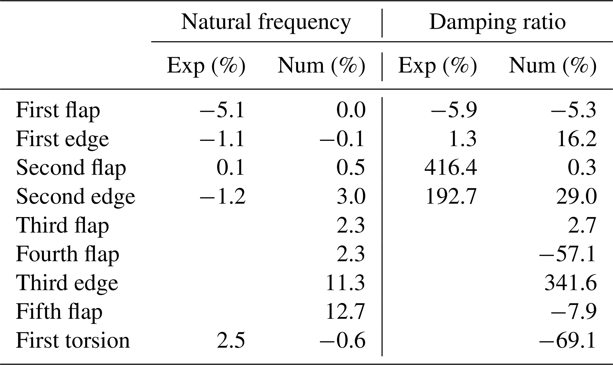
The verification comparing the natural frequencies predicted by the two numerical models shows that the frequencies up to the fourth flap, second edge, and first torsional modes match within 3 %, with negligible differences for the first flap, edge, and torsional modes. The validation step also shows a good match between the experimental results and the predictions of OpenFAST, with the exception of the first flap mode. Here, both models underpredict the natural frequency by 5.1 %. The research team could not explain the offset, which could have various origins, such as the impact of clamping of the blade root during laboratory testing.

The comparisons of structural damping show larger relative errors. Damping is an input to aeroelastic solvers, and it is modeled differently across frameworks. BeamDyn models damping as a set of six stiffness-proportional values accounting for three rotations and three translations. This allows the user to set the desired damping for a mode of interest, usually the first or the second. In this study, three values of flapwise, edgewise, and torsional damping were initially set based on the experimental data from GE to match the first modes. These values achieved differences of −5.9 % for the first flap mode and 1.3 % for the first edge mode. Because of the stiffness-proportional formulation, damping in the second modes was greatly overpredicted by OpenFAST compared to the results obtained in the laboratory. Despite this overprediction, the turbine in OpenFAST suffered from edgewise instabilities, which were resolved by artificially increasing the values of edgewise damping by almost an order of magnitude. The higher damping value is believed to compensate for some discrepancies in the unsteady aerodynamic solvers, which will be investigated in future work. Note that recent work has verified OpenFAST against other aeroelastic solvers, where there was no need to increase the edgewise term of structural damping (, ).

2.2.2 Elastic response of tower and drivetrain

While the elastic response of blades was modeled at relatively high fidelity, the tower of the turbine was modeled in ElastoDyn, which implements a reduced-order beam model using the first two tower fore–aft and side–side modes. The fore–aft and side–side stiffness distributions and unit mass distribution were specified according to values provided by GE. Note that ElastoDyn models the tower as torsionally stiff. Work is planned in OpenFAST to include tower torsion within its elastic model ElastoDyn. A workaround consisted of modeling the tower in the module SubDyn, but this was not pursued in this work. The verification step consisted of verifying numerically the tower mass, which matched exactly, and then the natural frequencies with and without the rotor nacelle assembly. The results for the first four tower modes, namely the first and second side–side and fore–aft modes, are reported in Table 2.

Table 2 Comparison of tower natural frequencies with and without rotor nacelle assembly (RNA) between OpenFAST and the numerical values shared by GE. The values provided are in terms of percent difference for the first four modes, namely the first and second side–side and fore–aft tower modes. Positive values represent higher frequencies in OpenFAST relative to the numerical values shared by GE.

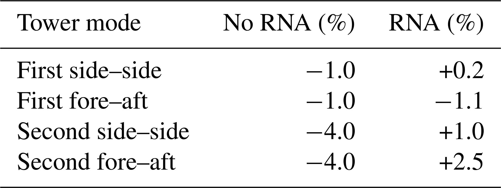
The comparison returned small discrepancies between natural frequencies by OpenFAST and natural frequencies by the numerical solver at GE. The discrepancies were attributed to the different model fidelity and to different discretization of the tower properties along its height. In terms of damping, the values for the tower structure were assigned to the individual modes.

OpenFAST currently models the drivetrain as an assembly of lumped masses. The only exception is the torsional stiffness and damping of the drivetrain system, which were populated thanks to data shared by GE. Sensitivity studies were conducted including the nodding and yawing flexibility of the nacelle in OpenFAST. Results were impacted to a negligible amount.

2.3 Aeroelastic response of the turbine system

Next, the aeroelastic modeling of the full turbine was verified and validated during turbine operation.

2.3.1 Experimental modal analysis

The experimental natural frequencies were obtained by calculating the power spectral density (PSD) for signals from strain gauges installed at the blade root and tower base. In signal processing, there are several ways of converting a signal from the time domain to the frequency domain. Choosing the correct method depends on the data or signals in question. In this scenario, Welch's averaged, modified periodogram method with a Hanning window was used to convert time-series data to the frequency domain. This method was preferred, as its approach to periodogram estimations helps reduce noise in the power spectra.

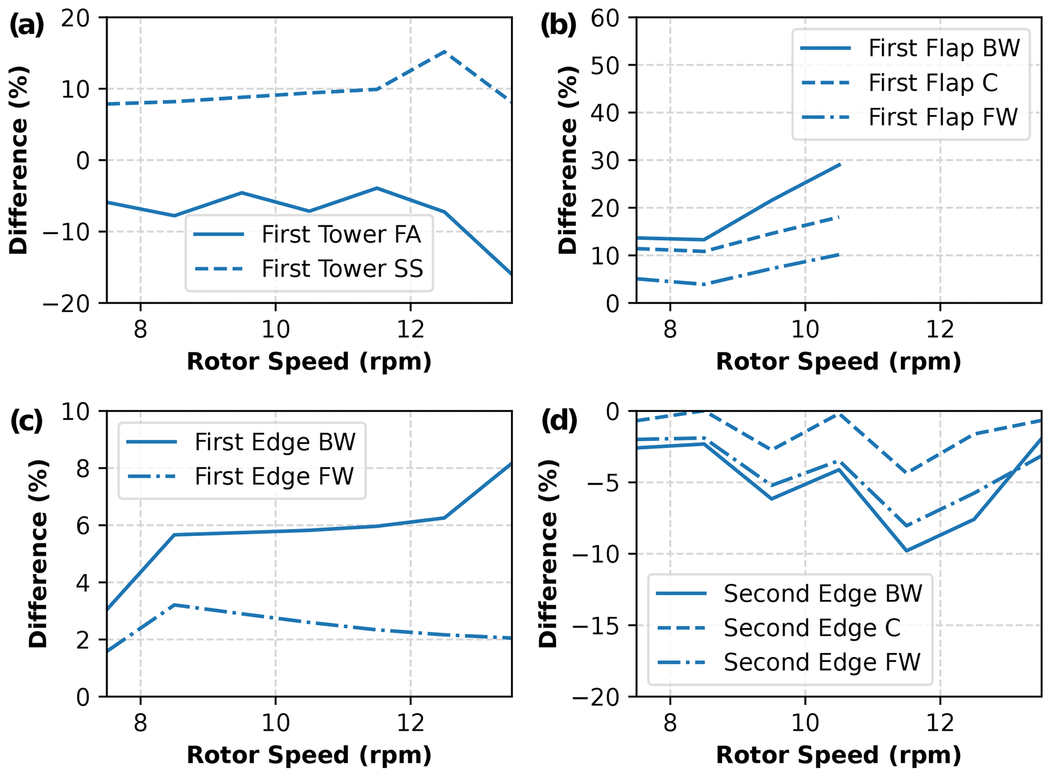
Figure 3 Relative differences between numerical (OpenFAST) and experimental (from strain gauges) natural frequencies for first tower modes (a), first rotor flap modes (b), first rotor edge modes (c), and second rotor edge modes (d). For the tower, fore–aft (FA) and side–side (SS) modes are reported. For the rotor, backward whirling (BW), collective (C), and forward whirling (FW) modes are reported. Positive values represent higher frequencies in OpenFAST relative to experimental values.

The analysis of the experimental data used for modal analysis was split into two sections: emergency stop and normal operation. Data from emergency stops were helpful for finding component natural frequencies by minimizing the impact of rotor aerodynamics. The normal operation data were binned by rotor speed between cut-in and rated. The analysis was limited to this range of wind speeds to conduct the comparison between experimental and numerical natural frequencies as a function of rotor speed, which only varies up to rated.

Conducting the experimental modal analysis with the existing set of installed sensors came with several challenges. A critical limitation was that the only measurement location along the blade span was the strain gauges close to the root. Therefore, it was not possible to extract any information regarding modal shapes. Fundamentally, the gauge measurements only allowed us to derive the PSDs of the blade-root strain.

When analyzing the PSD, it was found to be difficult to isolate and find the component frequencies. Consequently, the peaks were saturated and extremely challenging to identify experimentally, especially when we chose to run a blind comparison to the numerical model. It was particularly difficult to find the first and second blade-root flap frequencies during normal operation. We were only able to extract the first flap frequency from emergency stop data. This is not abnormal as the flap modes are typically strongly damped by the aerodynamics, which then leads to the difficulty of peak finding in the PSDs. Additionally, there was high uncertainty related to the second blade-root edge frequency because the peaks varied between data files, and there were instances where there was no energy in the expected region. We tried to apply a method known as time-synchronous averaging, which can help remove the rotor passing frequencies; however, this would have required a much higher data sampling frequency to be successful.

2.3.2 Validation of modal analysis

The relative difference between experimental frequencies extracted using the strain gauge data and the numerical frequencies estimated using OpenFAST is shown in Fig. 3 across a range of rotor speeds. For the first flapwise modes, we observe a good agreement at lower rotor speeds and growing discrepancies at higher speeds. Note that this trend is opposite to the one reported in Table 1, where OpenFAST underpredicts the natural frequency of the first flapwise structural mode. The different trend is attributed to limitations of the linearized unsteady aerodynamic model (see Sect. 2.1 and Branlard et al., 2022) and to the uncertainty in the high aerodynamic damping, which makes both numerical and experimental frequencies hard to identify. The numerical and experimental first and second edgewise modes match better, with differences within 10 %. The better match is explained by the small impact that rotor aerodynamics have on edgewise modes and by a more precise determination of the experimental frequencies of the system. Note that edgewise modes are more important than flapwise modes because they are usually affected by low damping and are prone to aeroelastic instabilities (Volk et al., 2020). Lastly, tower modes match within 10 % at low rotor speeds, growing to ± 15 % toward rated rotor speed. Again, the impact of aerodynamics is thought to be responsible for the growing offset.

2.4 Controls

While the ideal validation process would incorporate the actual turbine controller in the turbine model, such as in Zierath et al. (2016), this was not possible due to concerns around intellectual property. The solution to this problem was to adopt the ROSCO controller (Abbas et al., 2022), which was coupled to OpenFAST to match the steady-state and transient behavior of the field controller observed through historical SCADA data. The ROSCO generator speed set points were used to match those of the field controller. The peak-shaving, or thrust-limiting, parameter of ROSCO was used to reproduce the mean and peak blade and tower loading near rated power; this also resulted in similar near-rated power production. Step wind simulations were used to tune the transient response of the torque and pitch controller bandwidths to match the GE controller's response to the same wind input. For simplicity, we omitted pitch actuator dynamics and tuned the pitch response only using the controller gains of ROSCO. Modeling actuator dynamics would have added a tuning parameter and could have led to a better match, but the overall goal of tuning the pitch response of ROSCO to match the SCADA data would have remained the same.

Because of the long run times for OpenFAST simulations with BeamDyn, we ran 72 step wind simulations in parallel with uniformly distributed ROSCO tuning inputs (pitch and torque control bandwidths). We then evaluated the difference in generator speed and rotor thrust response between the GE reference and our controlled OpenFAST model. The simulation parameters with the lowest error were used to prescribe the parameters for another set of 72 simulations in a smaller design space. From these simulations, the best combination of low generator speed and rotor thrust error was used to select the set of ROSCO tuning parameters. Since both the generator speed and the rotor thrust error could not be simultaneously optimized, some judgment was used to give slightly more weight to the generator speed response error as it is a more direct measure of the controller's desired behavior.

Although available in ROSCO, individual pitch control (IPC) and tower damping control features were not enabled because the controller logic used to activate these features in the proprietary field controller was unknown. Even so, a generally good agreement between the field controller and ROSCO was realized, as is demonstrated in Sect. 4.1. Differences in the specifics of the implementation of the GE versus ROSCO controller, which cannot be disclosed, will lead to changes in transient behavior and could lead to small discrepancies in fatigue load results.

3 Inflow assimilation methods

This section describes how field data were used to generate one-to-one inflow bins for the numerical simulations.

3.1 Experimental campaign

The validation of the OpenFAST model presented here is based on measurements collected prior to the RAAW field campaign. The inflow and turbine measurements are therefore limited to instrumentation already present at the site before RAAW.

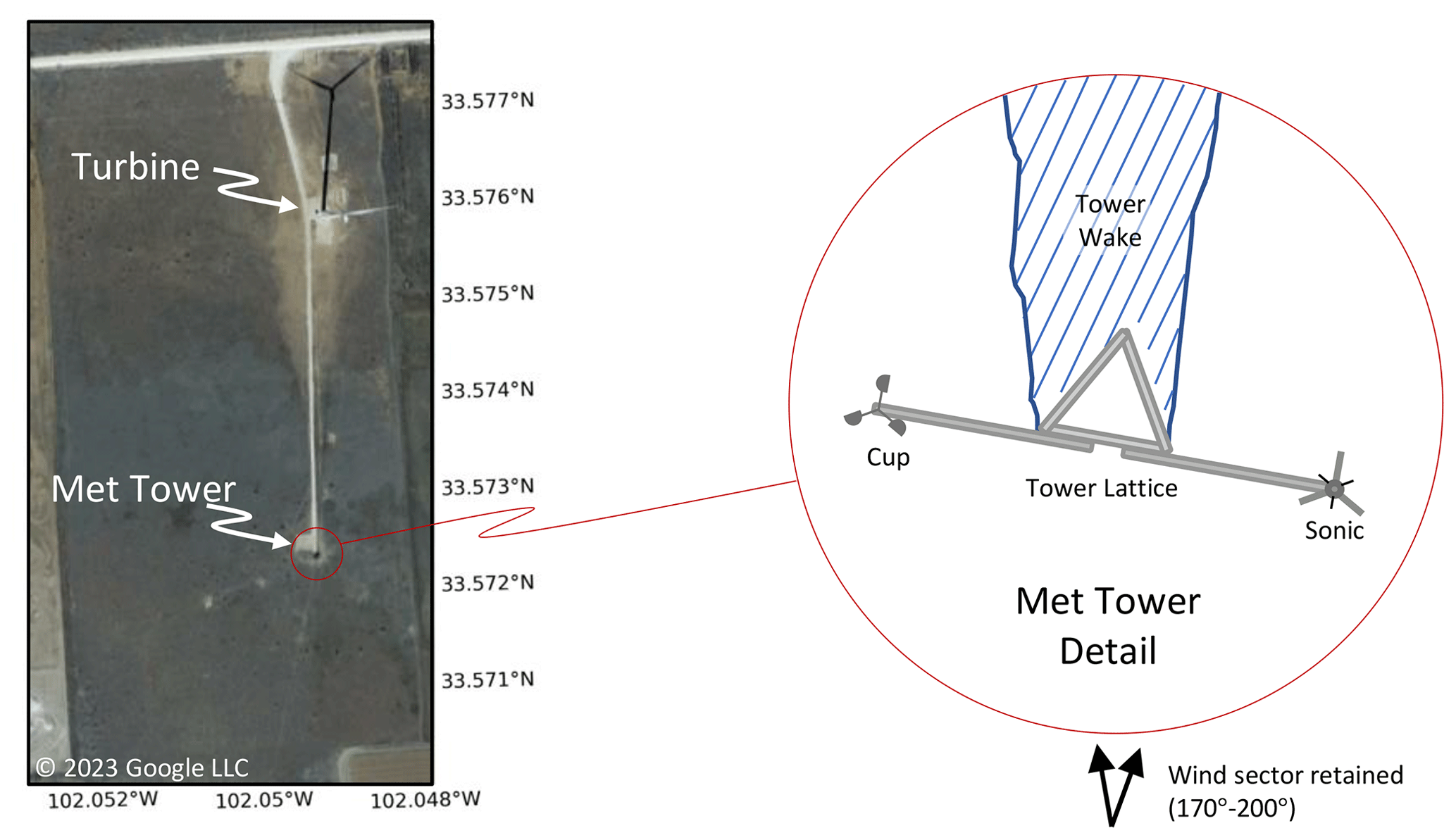
Figure 4 Planform view of the test site, including inset showing the cup and sonic anemometers in relation to the wake of the tower lattice for the wind sector retained in this study.

In terms of inflow measurements, we focused on assimilating data from the meteorological tower, which is shown in planform view in Fig. 4 along with the turbine. The meteorological tower was instrumented with various wind sensors, including three RM Young 81000 ultrasonic anemometers, five Thies Clima First Class cup anemometers, three MetOne 020WD wind vanes, and a ground-sitting WindCube lidar, the latter of which provided only 10 min statistics during the period considered here. In this study we preferred to use data from the ultrasonic anemometers rather than data from the cup anemometers with co-elevated wind vanes because of the inclusion of the w component of velocity in the ultrasonic measurement and because of a malfunction in the top-tip wind vane during the campaign. The 10 min WindCube data were used to remove static wind-direction offsets in the ultrasonic data that ranged between −9 and 14° between the various anemometers, likely due to misalignment during installation of the ultrasonics with the cardinal directions. The three ultrasonic anemometers spanned nearly the full height of the rotor and were mounted onto booms at 52.6, 110.5, and 179.5 m. The historical data analyzed herein were output at a frequency of 1 Hz (note that this value was later raised to 20 Hz for the continuation of the data collection happening within the RAAW experiment).

Related to measurements on the turbine, the layout of instruments on the turbine are shown in Fig. 5. In line with the objectives presented in Sect. 1, the wind turbine channels of interest for this study included the rotor speed, blade pitch, electrical power, and blade-root and tower-base bending moments, the latter two of which were sensed with strain gauges located near the blade roots and tower base, respectively. Re-calibrations of the strain gauges were performed such that the calibrations were never out of date by more than 90 d. Even so, we estimate an uncertainty of up to 150 kN m in these measurements based on changes in some of the calibrations over such intervals.

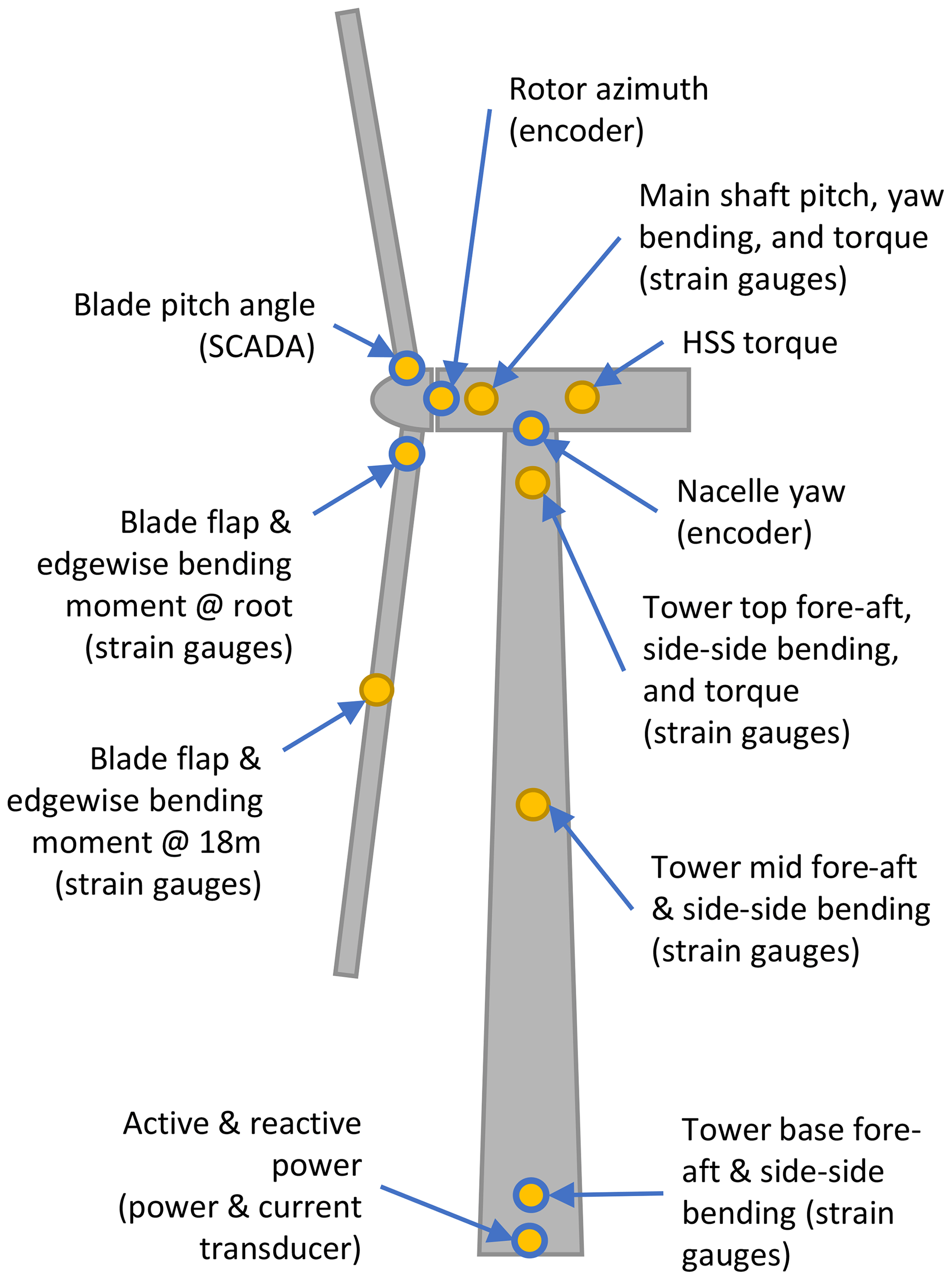
Figure 5 Illustration of instrumentation on the prototype wind turbine. The channels discussed in this article are outlined in blue.

The validation data in this article were collected between 22 September 2021 and 14 May 2022, and data are organized into 10 min bins during this period. For each bin, several preprocessing steps were applied to the ultrasonic data to render the data appropriate for model validation. First, following Kelley and Ennis (2016), who processed 2.5 years of meteorological tower ultrasonic data from the nearby 200 m tower run by Texas Tech University, several quality control filters were applied to the u, v, and w signals:

• remove all values above an absolute magnitude of 30 m s⁻¹;

• remove all values that are identically zero;

• remove all remaining values that are deemed spikes or statistical outliers in the time-series data, as identified using a median absolute deviation filter with a time window of 300 s and a threshold of 5 × 1.4826 = 7.4130.

An additional filter used in Kelley and Ennis (2016) to remove values based on a hold detection criterion was omitted from the current work since this filter appeared to be eliminating valid data in some cases.

Next, bins that had less than 95 % remaining data availability or had time spans of removed data longer than 5 s were also rejected. For the accepted bins, any instances of scattered data removal were filled in with a cubic hermite interpolation. Summary statistics were then calculated over 10 min bins. Finally, the horizontal components of the velocity series at each ultrasonic height were rotated into the reference frame of the 10 min mean reading of the hub-height wind vane, which was the appropriate form for input into the inflow assimilation methods.

In addition to the preprocessing steps above, the wind and turbine data of each 10 min bin also underwent several filtering processes to be deemed valid and useful for the validation analyses. These filters included bounds to eliminate bins that included malfunctioning sensors, bins with an idling turbine, bins including turbine start-up/shutdown events, bins with absolute mean yaw misalignment greater than 10°, bins with yaw standard deviation greater than 4°, bins with absolute mean shear exponent greater than 1, bins with absolute mean veer (as linearly fit from measurements taken from 52.6 to 179.5 m above ground level) greater than 50°, and lastly bins where the wind direction deviated more than 15° from the 185° heading of the meteorological tower relative to the turbine. This last condition not only prevented the ultrasonic sensors from ever being waked by the mounting boom arms, the meteorological tower structure, or the wind turbine, but it also meant that specific turbulence structures passing through the rotor disk were more likely to be the same as those sensed by the meteorological tower, assuming a frozen turbulence hypothesis.

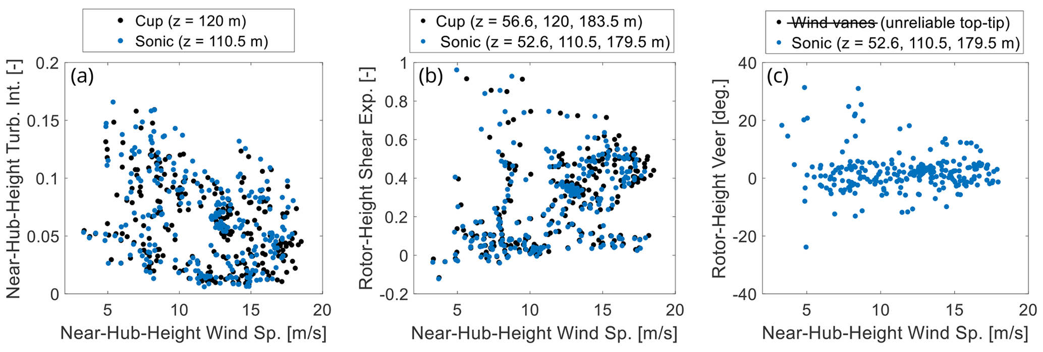
Figure 6 Mean inflow conditions for the 253 bins of 10 min selected for model validation: (a) horizontal turbulence intensity near hub height, (b) shear exponent calculated from a power-law fit over the rotor span, and (c) veer calculated from a linear fit over the rotor span. The data are plotted versus horizontal wind speed as measured by the ultrasonic anemometer near hub height (at 110.5 m).

The above filtering reduced the data set to 253 bins of 10 min, or 1.8 d, for validation analysis. Figure 6 displays 10 min inflow statistics from these bins, which demonstrate a diversity of inflow conditions and thus imply a relatively broad range of turbine operating conditions. The lack of cases with turbulence intensity above 0.15 in Fig. 6a is a consequence of the filtering on yaw standard deviation as described above, which was required because of limitations in the modeling setup. It is also noted that the existence of some relatively high shear exponents in Fig. 6b is a known characteristic of the site, and cases with these conditions were retained in the data set, though some validation error should be expected for such cases since IPC was not included in our turbine model while it was active in the field turbine in these cases. We elected not to filter such cases from the data set because many 10 min bins had some IPC activity but few bins had persistent IPC activity (some justification for this choice is provided in Sect. 4.3). Data for rotor-height veer from the wind vanes is omitted from Fig. 6c because of non-physical wind-direction shifts that were observed in the readings of the wind vane near the top-tip position. However, the wind vane near hub height, which was used to rotate the ultrasonic data into the appropriate reference frame as described previously, was reliable.

3.2 Computational environment

The inflow simulations were performed in three different ways by using two different sets of inputs to TurbSim (Jonkman, 2014) as well as an implementation of PyConTurb (Rinker, 2018). These kinematic turbulence generators begin with information on the spectra and spatial coherence of velocity components, which are then translated to the time domain via an inverse Fourier transform. Each generator can produce Gaussian turbulence fields according to a spectral model, which is herein taken as the Kaimal spectrum with exponential coherence as defined in the International Electrotechnical Commission's (2005) 61400-1 standard.

Table 3 Comparison of inflow assimilation methods. Single-point constraints are enforced from the ultrasonic anemometer near hub height (i.e., z = 110.5 m), and three-point constraints are enforced from all three ultrasonic anemometers.

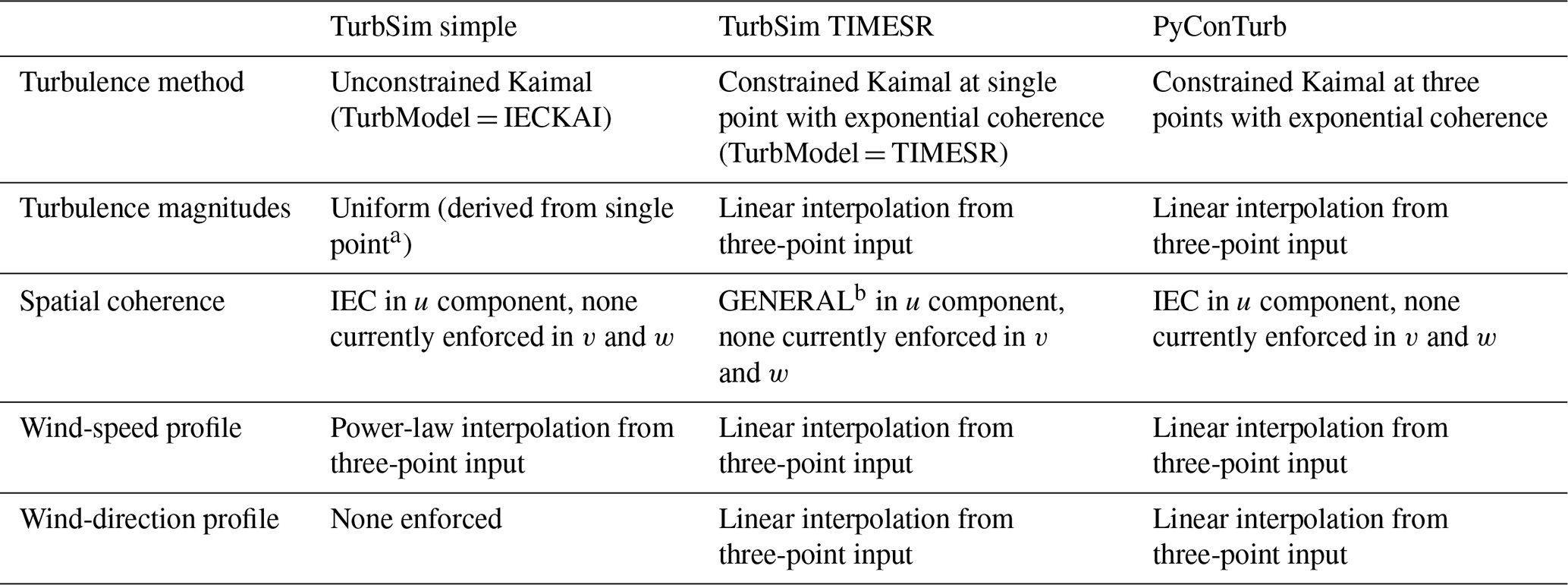
^a The near-hub-height velocity time series is linearly detrended before calculating turbulence intensity as per Larsen and Hansen (2014), and the input field ScaleIEC is set to 1 to enforce the exact value specified near hub height given the desired sample rate. ^b See Jonkman (2014) for a description of the coherence model.

The differences among the three approaches, which are described in Table 3, center around how the measured data are assimilated. The turbulent fluctuations in the baseline TurbSim approach, termed here TurbSim simple, are stochastic and based on the turbulence intensity measured by the ultrasonic anemometer at the near-hub-height location. The Fourier magnitudes are determined from the spectral model, which is scaled so that the turbulence intensity matches that which was specified. Random phases are applied to the Fourier terms, and the phases of the streamwise component of velocity are correlated based on the spatial coherence model. The two higher-fidelity approaches of generating inflow are TurbSim with the TIMESR option and PyConTurb. These two approaches constrain the turbulent time series to match time-resolved measurements by linearly interpolating Fourier magnitudes from the measured time series to the computational grid and constraining the Fourier phases to match the wind series provided at one or more measurement locations. In TurbSim TIMESR, only one point in the domain can be constrained. PyConTurb, in contrast, is able to apply the same constraints to an arbitrary number of points. For the simulations performed here, TurbSim TIMESR is constrained based on the near-hub-height ultrasonic anemometer measurements. In PyConTurb, all three ultrasonic anemometer measurement locations are used. For each turbulence assimilation method and each 10 min bin, six turbulence seeds were generated to improve statistical convergence over the non-constrained data of the turbulence grids. As a result, 4554 turbulent inflows were produced (253 bins of 10 min, six random seeds, and three different approaches).

Other differences between the three methods are related to how the mean wind speed and direction are assimilated from the measurement. As shown in Table 3, TurbSim simple has the most restrictive assumptions in this regard, as it only generates power-law wind profiles without veer. The two other methods are more flexible, though the linear interpolation of wind data for these methods is likely to result in wind-speed and wind-direction profiles that do not exactly match the observed conditions, especially in stably stratified conditions.

For all three methods, the turbulence plane was a lateral–vertical grid of 33 by 33 points that was 10 % wider than the rotor diameter both laterally and vertically (see Fig. 7). The TurbSim methods include tower nodes to simulate wind loading on the entire tower including the region below the turbulence plane (Jonkman, 2014), whereas PyConTurb does not have this feature. Tower aerodynamics were therefore disabled for the PyConTurb cases.

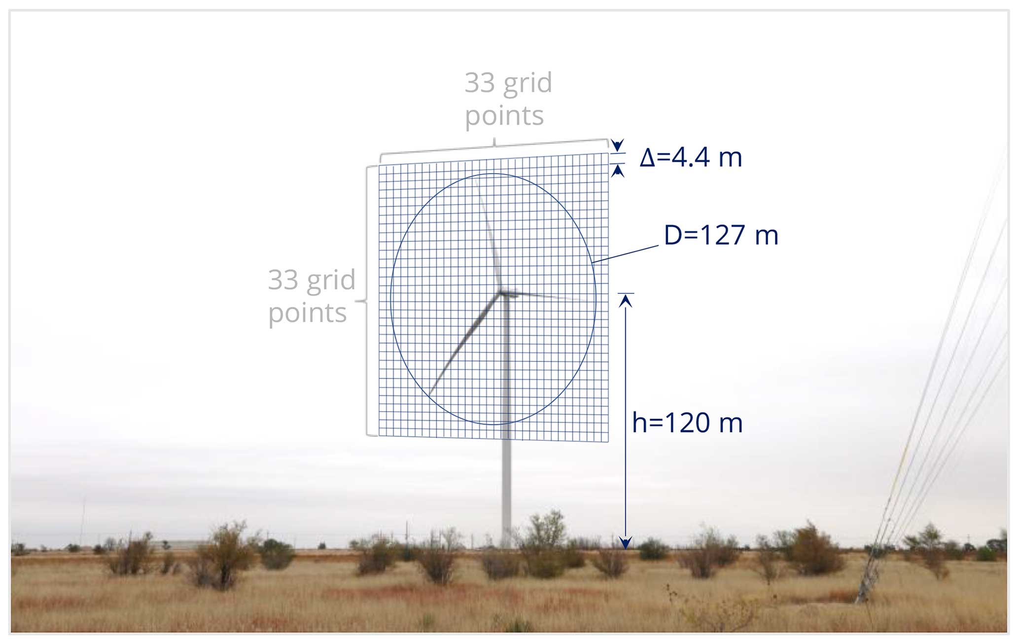
Figure 7 Image of the 2.8 MW GE wind turbine in Lubbock, Texas, USA, with turbulence grid overlaid.

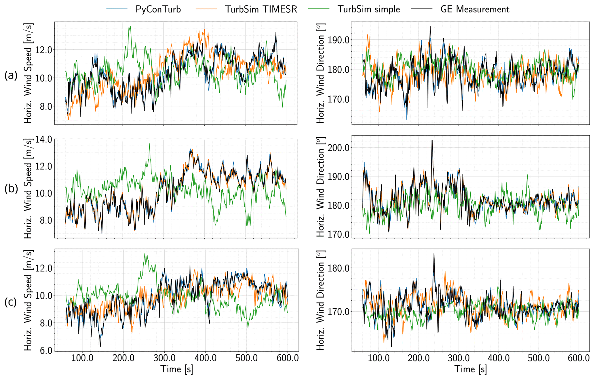
Figure 8 Comparison of time series of simulated inflow to measured inflow for an example 10 min bin for the sonic anemometers near (a) top tip, (b) hub height, and (c) bottom tip. The simulated data have been interpolated from the computational grid to the exact measurement locations, which were 179.5, 110.5, and 52.6 m, respectively. Only one of six turbulence seeds is shown.

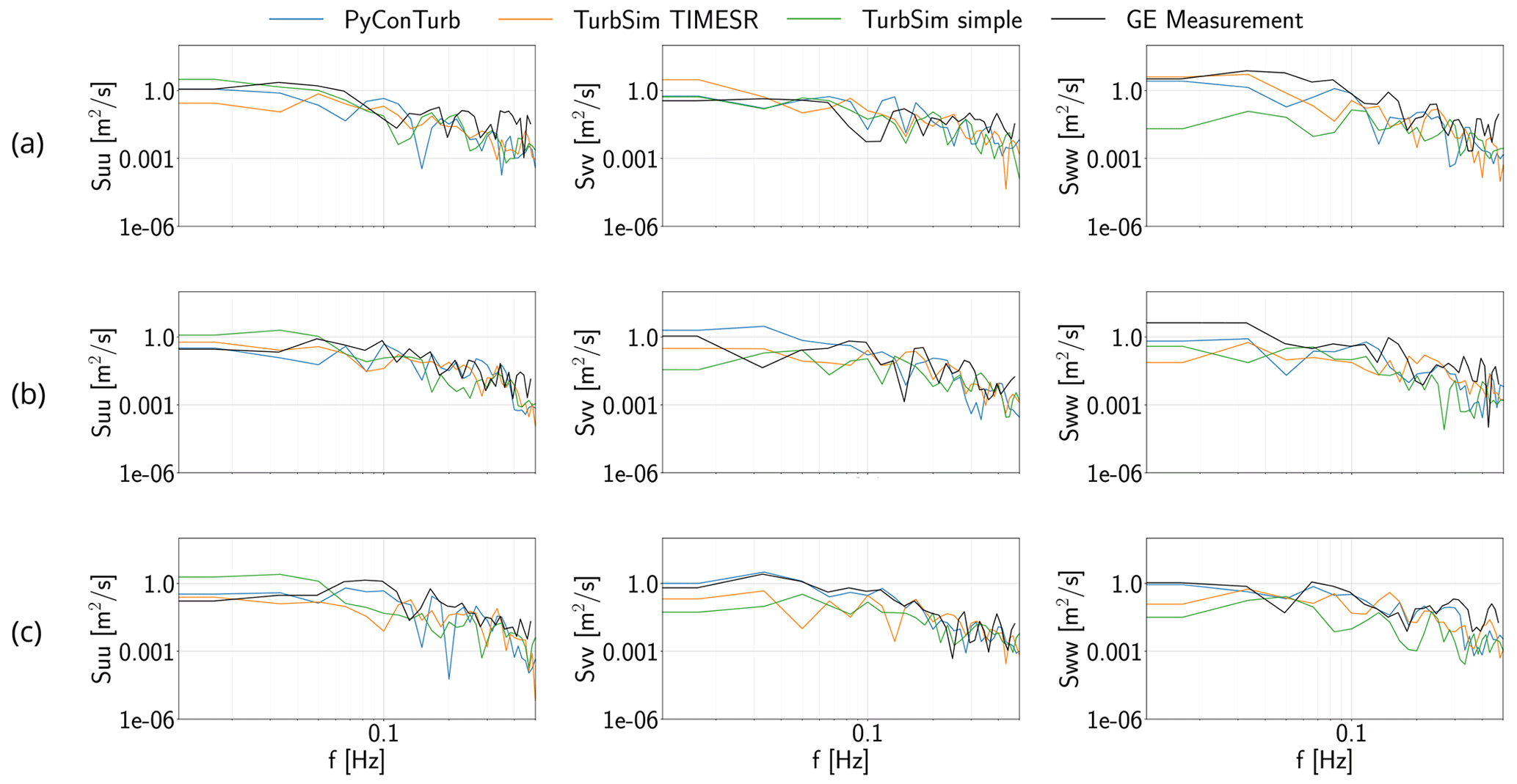
Figure 9 Comparison of turbulence spectra of simulated inflow to measured inflow for an example 10 min bin for the sonic anemometers near (a) top tip, (b) hub height, and (c) bottom tip. Before calculating the spectra, the simulated data have been interpolated from the computational grid to the exact measurement locations, which are 179.5, 110.5, and 52.6 m, respectively. Spectra are calculated with the one-sided welch method using 60 s bins and a Hanning window. Only one of six turbulence seeds is shown.

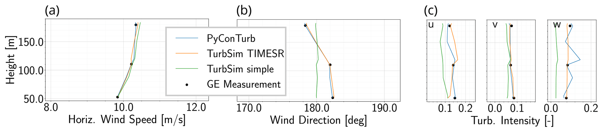
Figure 10 Comparison of vertical profiles of simulated inflow to measured inflow for an example 10 min bin for (a) horizontal wind speed and (b) direction, as well as (c) the three components of turbulence intensity, which are calculated as the standard deviation of the given component divided by the mean of the u component. Only one of six turbulence seeds is shown.

Figures 8, 9, and 10 show an example of the simulated inflow versus the measurement for an example 10 min bin captured on 16 March 2022. The data here illustrate that TurbSim simple generally matches only the 10 min statistics, while the constrained turbulence assimilation methods (i.e., TurbSim TIMESR and PyConTurb) additionally match the time-varying values at one or more measured heights. The small differences in the data of TurbSim TIMESR and PyConTurb compared to the measurement at the constraint points are due to non-alignment of the simulation grid with the measurement location, and PyConTurb notably has two more constraint points than TurbSim TIMESR, as illustrated by matching of the measurement data by PyConTurb at the near-top-tip and near-bottom-tip positions as well as the near-hub-height position. Note that the detrending process for TurbSim simple described in the footnotes of Table 3 results in significantly lower turbulence levels for TurbSim simple in this (and some other) bins because of the time gradient in wind speed during this interval. The corresponding difference in turbulent energy does not manifest in the spectral plots of Fig. 9 because the data have been binned on 60 s intervals, thus eliminating the long-pass timescale that is affected by the detrending process.

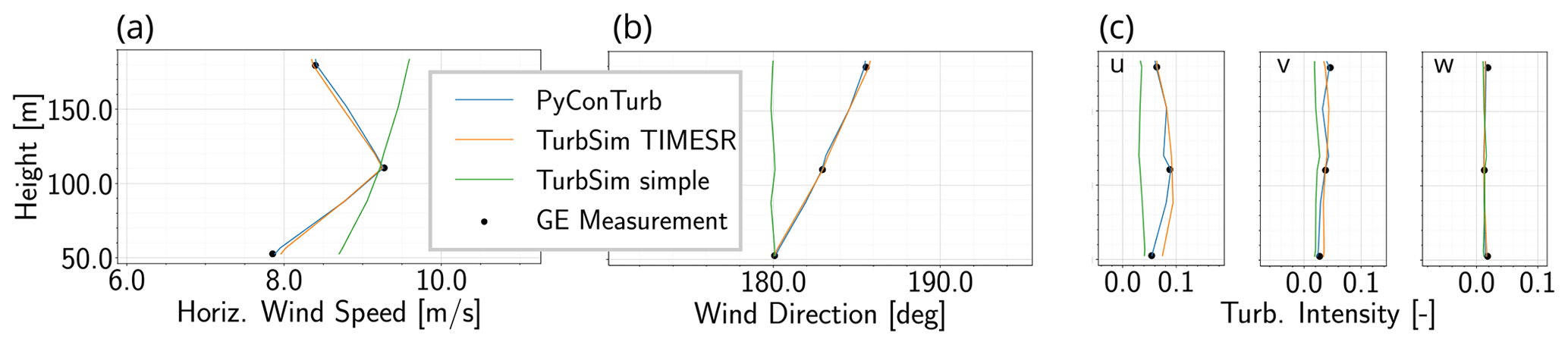
Figure 11 Analog to Fig. 10 except for an example 10 min bin that includes a non-monotonic shear profile.

For reference, the 10 min statistics of another example bin are given in Fig. 11. This bin demonstrates a non-monotonic shear profile (i.e., jet) that is sometimes observed at the site. TurbSim simple is not able to capture the shape of the shear profile, whereas the two higher-fidelity approaches can roughly capture the shape within the limitations of linear interpolation.

A note is appropriate about the frequency of the wind field input to OpenFAST, which is unaltered from the 1 Hz sampling frequency of the meteorological tower described previously. For calculations involving DEL, neglecting frequency content in the wind higher than 1 Hz will lead to slight underprediction of DELs. For a turbine of similar size and rated rpm, Sim et al. (2012) demonstrate an underprediction of 5 % and 2 % for the blade-root flapwise DEL and tower-base fore–aft DEL, respectively, by using a 1 Hz inflow and a coarse turbulence grid compared to an inflow with higher temporal and spatial resolution. In this study, we make no attempt to populate the higher-frequency content of the measured inflow but note that the measured 1 Hz corresponds to more than 4 times the rotor revolution frequency (> 4P) at rated rpm, which allows excitation of the 3P frequency. Frequencies of 6P and 9P, which might especially affect the tower, are not present in the simulation at rated rotor speed.

3.3 Postprocessing

Outputs from the field turbine and simulated turbine were processed similarly. The first minute of each 10 min bin was discarded to remove transients in the simulated results. A temporal offset was then applied to the simulation time series to account for the advection time of the flow between the meteorological tower and the rotor by leveraging knowledge of the location of the meteorological tower relative to the turbine and by assuming the flow advected with the 10 min mean wind direction and speed as measured from the near-hub-height sonic anemometer on the meteorological tower. Both the experimental and simulation results were therefore shortened by 20–100 s depending on the wind speed so that only the overlapping segments of time between the simulated and measured channels were retained. After the temporal alignment process, bending moment data from the simulations were interpolated to the position of the strain gauges at the blade roots and tower base. Lastly, statistics including averages and DELs were calculated for each bin, and the latter was calculated as in the OpenFAST Python toolbox (Branlard et al., 2023) at a frequency of 50 Hz, which was the rate of the measurement and simulation output.

4 Results

This section describes the results of the one-to-one validation beginning with analysis of the basic operability (i.e., mean rotor speed and blade pitch) and proceeding to power, blade loading, and tower loading.

In the following subsections, the individual 10 min bins have been sorted into wind-speed intervals of 1.5 m s⁻¹ based on the mean horizontal wind speed of the ultrasonic anemometer near hub height. A histogram of the counts at each wind speed is shown in Fig. 12. As the rated wind speed is ∼ 11 m s⁻¹, there are roughly an even number of counts corresponding to above-rated wind speeds (i.e., Region III) as there are corresponding to below-rated conditions (i.e., Region II).

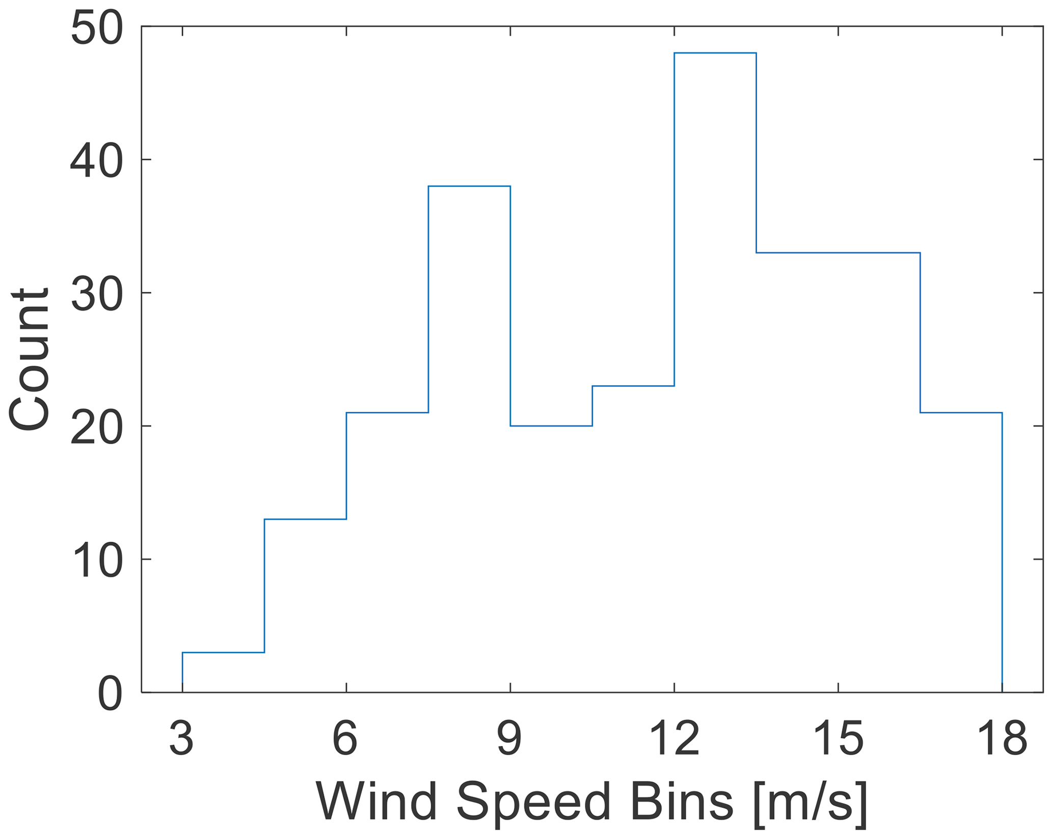
Figure 12 Histogram of the number of 10 min bins within each of the wind-speed intervals used throughout Sect. 4

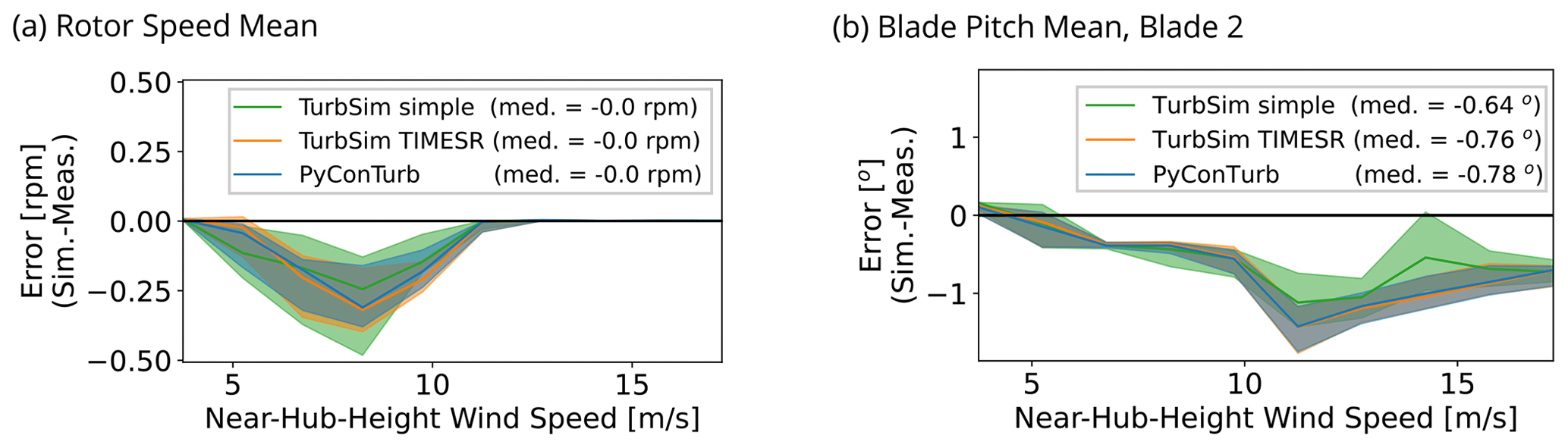
Figure 13 Comparison of (a) mean rotor speed and (b) mean blade pitch between models and measurement. The plots consist of statistics calculated within each wind-speed interval including the median (solid lines) and interquartile range (shaded areas). The median value reported in the legend is the overall median error calculated across all 10 min bins.

4.1 Basic operability

First we considered the basic operability of the turbine models in terms of the controller set points for rotor speed and blade pitch. Figure 13 shows statistics of the model errors over the 253 bins of 10 min compared to the measurements for rotor speed and blade pitch. For the rotor speed, the median errors within each wind-speed interval are less than 0.5 rpm, or within 4 %. This error is not very sensitive to the inflow assimilation method, though the spread of error (i.e., the interquartile range) is smaller for the higher-fidelity assimilation methods. For the blade pitch, all the inflow assimilation methods underpredict pitch above rated wind speed. The cause for the underpredicted pitch by all three models in Region III could be related to aerodynamic modeling errors that produce an underestimation of the aerodynamic torque.

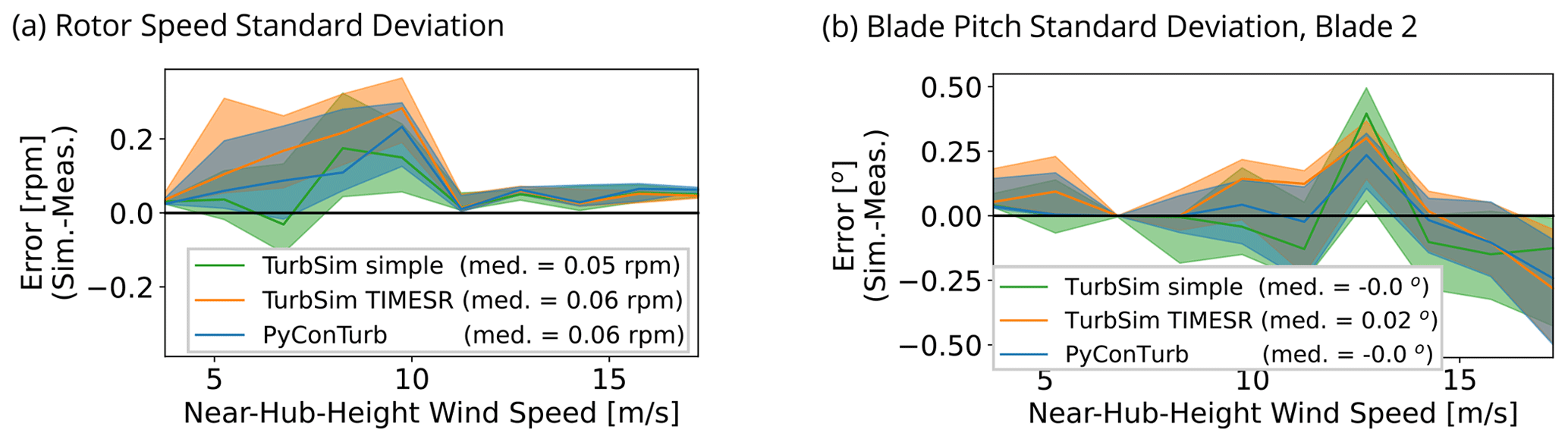
Figure 14 Comparison of (a) standard deviation of rotor speed and (b) standard deviation of blade pitch between models and measurement. See Fig. 13 for explanation of the lines, shading, and legend.

Figure 14 is analogous to Fig. 13 except it shows errors in the standard deviation rather than the mean. The median error in the standard deviation of rotor speed is less than 0.3 rpm, or 2 % of the nominal rotor speed at rated. The maximum error in the standard deviation of blade pitch is around 0.5°. Note that the underprediction of the standard deviation of blade pitch at wind speeds ≥ 14 m s⁻¹ appears to be a result of the omission of an IPC model in the controller, but the relatively small overall magnitude of the errors in this quantity corroborates the previous statement that few of the 10 min bins had persistent IPC activity in this data set.

4.2 Power

Figure 15 shows the comparison of simulated-to-measured power. The scatterplot in Fig. 15a indicates generally good performance of the models with increased scatter apparent below 10 m s⁻¹ that could be related to, for instance, spanwise inhomogeneity in the inflow that cannot be captured by the vertically aligned met tower sensors. In addition to the scatter, Fig. 15b reveals a negative bias in the median modeling error in Region II that is up to 8 % for the higher-fidelity inflow assimilation methods and 10 % for the simpler method. The source of the bias is not presently known but could plausibly be related to errors in modeling of the controller, blade twist, airfoil performance, or rotor aerodynamics. We note also that the underprediction of the models at the knee of the power curve may be a result of exaggerated modeling of the peak-shaving strategy of the proprietary field controller.

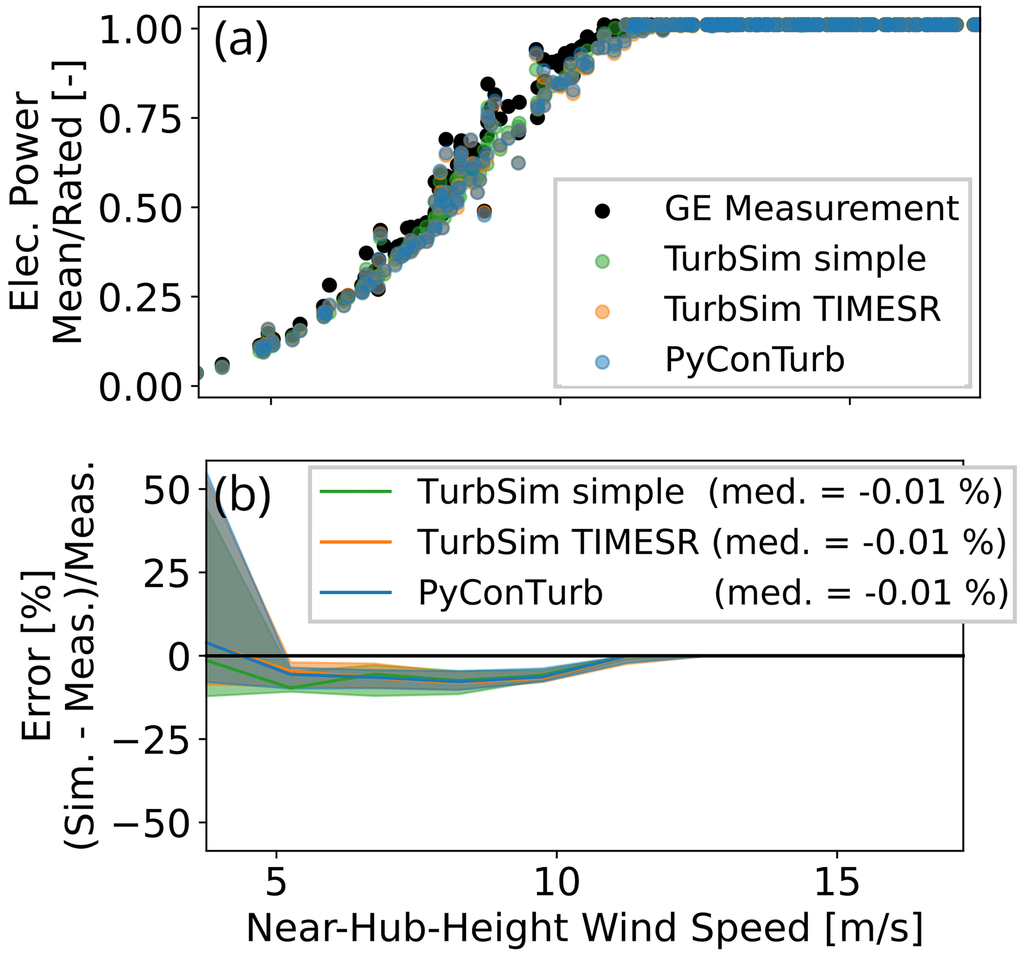
Figure 15 Comparison of (a) mean electrical power and (b) mean electrical power error between models and measurement. Each dot in panel (a) represents a 10 min time series. See Fig. 13 for explanation of the lines, shading, and legend in panel (b).

Figure 16 Comparison of (a, b) flapwise and (c) edgewise bending moment QoIs for blade 1 at 1.25 m from the root. See Fig. 13 for explanation of the lines, shading, and legend.

4.3 Blade loading

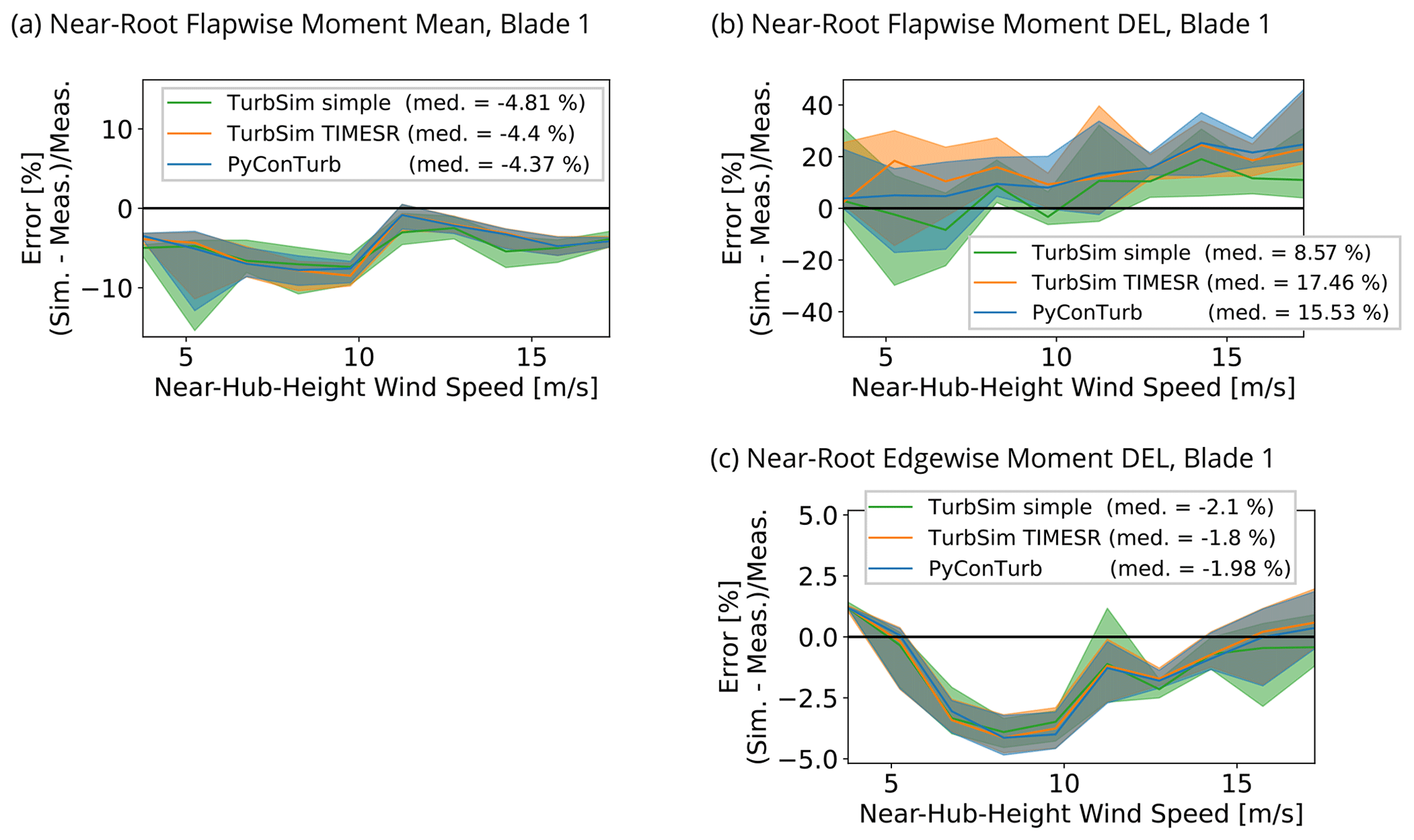
Figure 16a shows the near-root flapwise moment mean at blade 1. The comparison shows that median modeling errors in each wind-speed interval are within 10 %. The mean near-root edgewise moment is close to zero and is not reported.

The comparisons of the near-root DELs are shown in Fig. 16b and c. The edgewise comparisons in Fig. 16c show little sensitivity to the inflow assimilation method, which is congruous with Rezaeiha et al. (2017), whose study demonstrated that aerodynamics (i.e., turbulence, wind shear, and yaw) account for < 20 % of lifetime equivalent fatigue loads in the edgewise direction. Rather, it is rotor imbalances and gravity that dominate the edgewise fatigue budget. Thus, the < 5 % simulation error for edgewise DEL suggests that the blade model development in Sect. 2.2 was successful in terms of edgewise characteristics, granted the need to artificially increase the value of structural damping in the edgewise direction compared to the value assumed by GE Vernova, and this difference should be investigated further. Unlike the edgewise case, the flapwise fatigue comparison shown in Fig. 16b shows significant errors on the order of 8 %–18 % for the overall medians.

Figure 17 Comparison of the flapwise bending moment DEL from Fig. 16b except plotted versus (a) near-hub-height turbulence intensity and (b) rotor-height wind shear exponent. See Fig. 13 for explanation of the lines and shading.

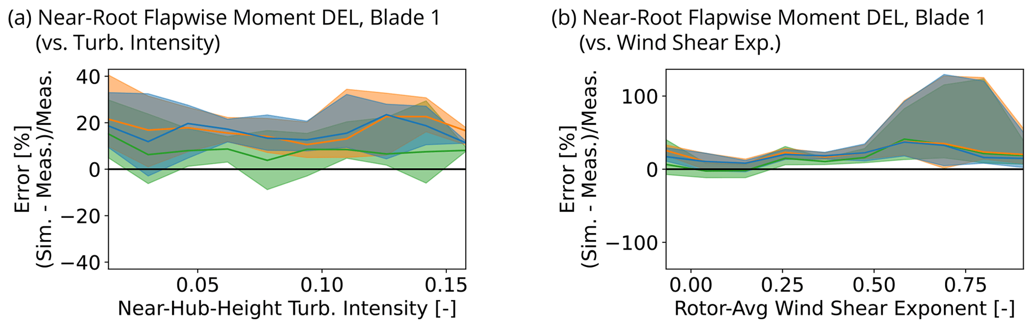
Given the magnitude of the model errors for the flapwise DELs, a closer investigation is warranted. The results from Rezaeiha et al. (2017) for a turbulence intensity similar to the mean of our study (i.e., ∼ 8 %) show that around half of the contribution to flapwise lifetime equivalent fatigue loads was from turbulence, and more than 8 % was from wind shear. Figure 17 replots the modeling error for flapwise DEL observed in Fig. 16b but this time as a function of inflow turbulence intensity and wind shear exponent. The flapwise DEL error has little correlation with turbulence intensity as shown in Fig. 17a. However, the flapwise DEL error shows a positive correlation with wind shear exponent, at least until the very highest shear exponents where the sample size is small. Several possible explanations for this trend are proposed.

The omission of modeling of the field turbine's IPC actions could produce this trend since IPC has been shown in some cases to reduce flapwise DELs on the order 10 %–20 % (Bossanyi, 2003; Van Engelen and Van Der Hooft, 2005). Indeed, the flapwise DEL errors fall closest to zero for all three inflow assimilation methods as the inflow shear exponent (and thus the likelihood of IPC activity) tends to zero. More specific insight on the effect of IPC on the flapwise errors in this data set can be gained by an additional filtering step as described next. One indicator of the strength of IPC activity is the standard deviation of the difference of two blades' pitch signals. Filtering out the half of the 10 min bins with the larger standard deviations and recomputing the error metrics only reduced the range of overall median flapwise errors reported in Fig. 17a from 8.57 %–17.46 % to 7.78 %–14.43 %. This result suggests that the omission of IPC in the models may not sufficiently explain the errors in the flapwise DEL predictions.

Another possible explanation is that overprediction of flapwise DELs stems from the computation of induction in OpenFAST. The last 10 years have seen awareness of overprediction of some unsteady QoIs from BEMT models versus higher-fidelity approaches, especially in sheared conditions (Madsen et al., 2012; Boorsma et al., 2016; Perez-Becker et al., 2020; Madsen et al., 2020). Although this overprediction seems to be improved by computing induction locally around the azimuth rather than using an annulus-averaged approach (Madsen et al., 2012, 2020), Perez-Becker et al. (2020) suggest that such locally computed induction fields as found in OpenFAST, which include induced velocities from bound and wake vorticity, are still not accurate. They observed the 1P fluctuations of the local angle of attack in OpenFAST to be overpredicted and found OpenFAST to consequently predict 9 % higher lifetime DELs for the out-of-plane blade-root and the tower-base fore–aft bending moments compared to a lifting-line free-vortex method. It might be argued that such an induction-related rationale is weakened in our case because the errors in flapwise DEL persist and even increase at higher wind speed where induction begins to decrease, but it is noted that the data in Fig. 6b show a correlation between the inflow wind speed and shear exponent.

In addition to the uncertainty surrounding the cause of the error in the flapwise DEL predictions, there also exists significant sensitivity of the error to the inflow assimilation method, which is not surprising given the aforementioned sensitivity of flapwise DELs to turbulence and wind shear and the fact that turbulence and wind shear are handled uniquely in each method. Considering the error as the wind shear goes to zero may give an indication of the performance of the models apart from the possible modeling errors related to IPC and induction noted above. Extrapolating the results in Fig. 17b to the point of zero wind shear suggests that the simplest inflow assimilation method (i.e., TurbSim simple) validates better than the higher-fidelity methods in terms of flapwise DELs. The apparent reason for the lower flapwise DEL predictions of TurbSim simple is the notably lower turbulence intensity of this approach stemming from the detrending process (see Figs. 10c and 11c and the first footnote of Table 3), which is believed to be good practice. Pedersen et al. (2019) found a similarly surprisingly result when comparing unsteady QoIs between simulations with unconstrained and constrained turbulence from a meteorological tower, and they concluded that measurements taken at large distances from the turbine should not be used to constrain turbulence because of possibly invalid assumptions related to frozen turbulence between the inflow measurement and turbine and those related to the measured flow field passing completely through the rotor disk. In our data set, the results from Region II in Fig. 14a and Region III in Fig. 14b (before 14 m s⁻¹ when IPC actions in the field turbine increase) indicate an overprediction of unsteadiness in the turbine set points. A hypothesis is that this added unsteadiness as well as a portion of the flapwise DEL overprediction could therefore be related to the BEMT formulation, which, in contrast to how the formulation modifies the mean velocity with a rotor induction model, does not account for changes to the relative magnitude of the fluctuating component of the velocity (i.e., distortion of turbulence structures) due to the induction field of the rotor. Branlard et al. (2016) and Mann et al. (2018) consider this question, and their conclusions about the degree of amplification or attenuation of the turbulence spectrum due to the presence of the rotor vary depending on the turbulent length scale and the region of rotor operation (i.e., the slope of the thrust coefficient curve versus wind speed). Further insight on this possible modeling discrepancy might be afforded by a higher-fidelity modeling technique such as a free-vortex wake method.

The combination of potential modeling errors discussed in the above paragraphs could be responsible for the observed error in the flapwise DELs, and the possible presence of compensating errors in the TurbSim simple method should be acknowledged, considering the lower overall errors for this inflow assimilation method compared to the supposedly higher fidelity constrained methods. Such errors could be related, for instance, to TurbSim simple using a uniform profile of turbulence magnitude drawn from the near-hub-height measurement, which would artificially lower the rotor-averaged turbulence intensity compared to a turbulence profile with higher curvature near the bottom tip than the top tip. Also, the use of a pre-defined spectral model in TurbSim simple leaves open the possibility that the energy content at the lowest frequencies of the turbulence spectra is on average too low compared to a spectra derived from time-resolved measurements. TurbSim simple also does not include effects of non-monotonic shear profiles (see Fig. 11a) or veer (see Fig. 11b) that would affect unsteady flapwise loading.

Another perspective on the flapwise DELs is offered by comparison of time series of flapwise loading for three time segments in Fig. 18. The effect of the time-offsetting process described in Sect. 3.3 is evident for the two constrained turbulence assimilation methods, which are able to more faithfully reconstruct the variations in blade loads on the longer timescales. The generally larger amplitude of the oscillations in the modeled results than the measured ones is consistent with the overprediction of flapwise DEL discussed above.

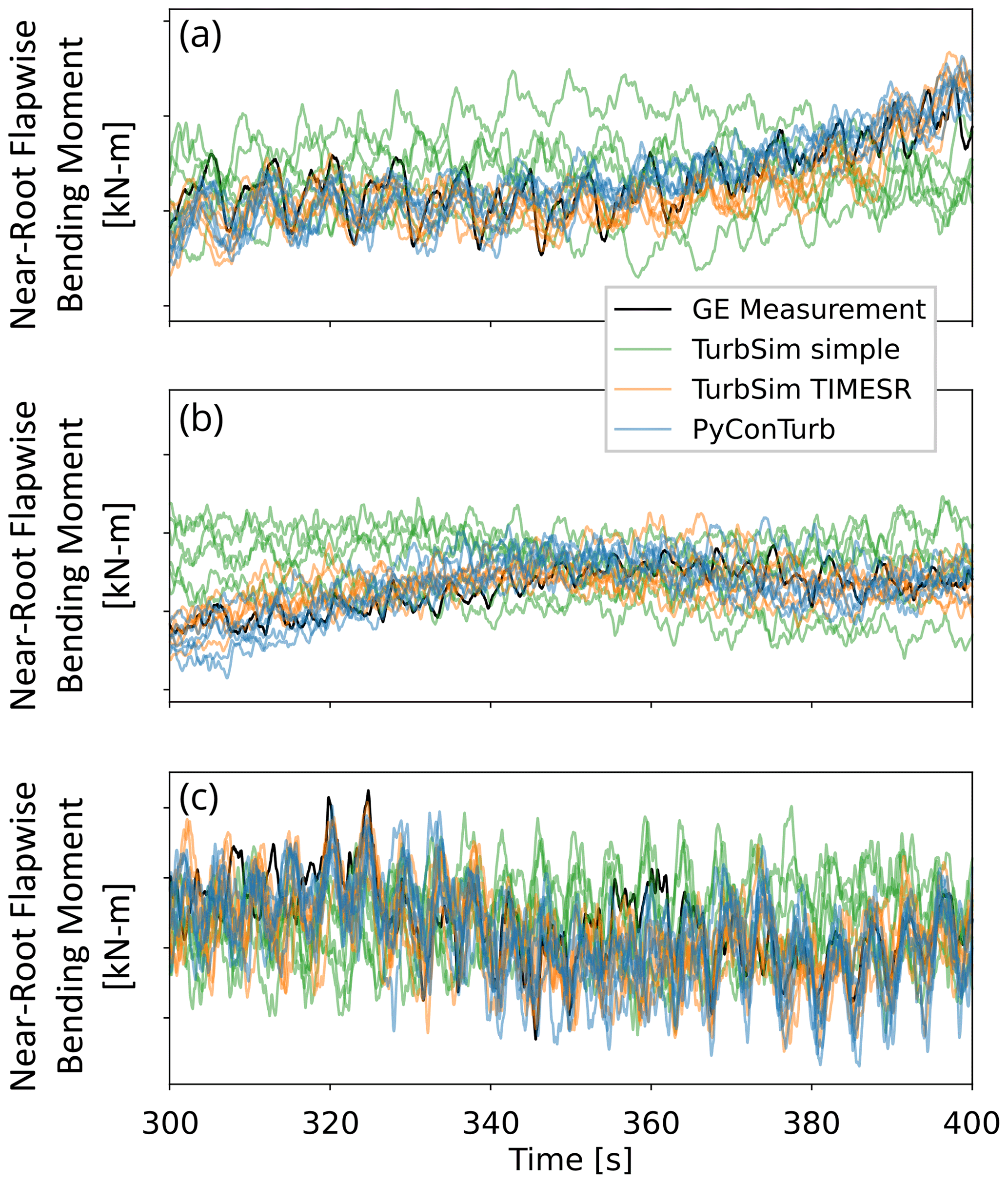
Figure 18 Comparison of time series of blade-root flapwise moment between measurement and simulation for blade 1. Each color of simulation data has six lines corresponding to the six turbulence seeds.

Figure 19 Comparison of fore–aft bending moment QoIs for the tower at 8.6 m from the base. See Fig. 13 for explanation of the lines, shading, and legend.

4.4 Tower loading

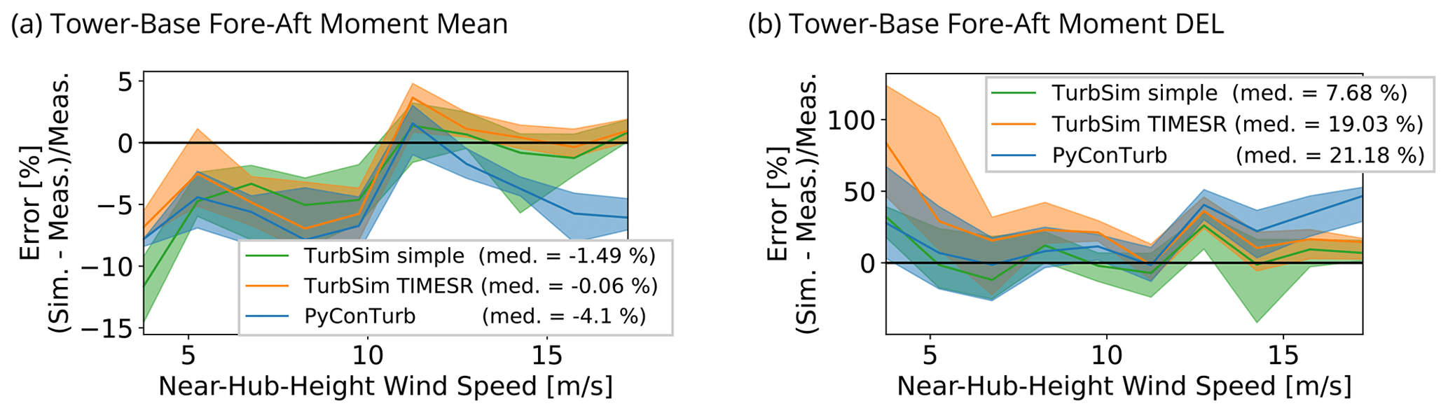
Figure 19 shows the comparison of tower-base bending moments. The median errors of the model in Fig. 19a are generally less than ± 10 % and indicate that the steady loading on the rotor and tower are well modeled, granted the underprediction of steady tower loading in Region II that is related to the underprediction of mean flapwise loading in this region as noted above. Note that the more negative mean error for the PyConTurb cases compared to the TurbSim ones is a result of the absence of tower nodes and tower aerodynamics in PyConTurb as described previously, and this effect grows with wind speed. The DEL errors of the model in Fig. 19b have a significant positive bias similar to that of the flapwise DEL errors. As before, the two higher-fidelity models show higher bias than TurbSim simple.

Similar hypotheses can be made for the overprediction of tower fore–aft DEL as for the overprediction of flapwise DELs in Sect. 4.3. The median errors for the fore–aft DELs in some wind-speed intervals are even larger than those for the flapwise DEL and could be related again to omission in the simulations of certain control features on the turbine, including collective-pitch tower damping, which could explain the local peak in DEL error near rated power. Another culprit for the large fore–aft DEL overprediction could be omission of the modification of the inflow turbulence by the BEMT model as suggested previously since the tower-base fore–aft DELs are known to be highly sensitive to the accuracy of the wind spectrum (Nybø et al., 2021).

5 Suggestions for a future validation campaign

Below are recorded lessons from the preceding analysis that may aid the design of future validation studies.

5.1 Inflow measurements

This study leveraged meteorological tower data to define turbulence grids. Shortcomings of this approach include low spatial resolution and negligence of the effects of the rotor induction on the characteristics of the inflow fluctuations. An improved experiment might include on-blade pressure probes as in Pedersen et al. (2019) to validate the induction physics predicted by the model. Taking a series of measurements as the flow moves toward the rotor, such as with a nacelle- or hub-mounted lidar, could additionally allow for step-by-step tracking of the inflow spectrum, shear, and veer, as well as comparison thereof with the same quantities predicted by BEMT models.

5.2 On-blade measurements

Further, on-blade surface pressure measurements would be useful to quantify errors related to airfoil polars and three-dimensional effects. Tracking of the level of soiling on the turbine blades during the measurement period might also lead to more informed selection of the roughness condition of airfoil polars to be used in models. Better information about the local blade aerodynamic behavior will lead to improved estimates of aerodynamic frequencies and damping.

5.3 Experimental modal analysis

From the initial modal analysis discussed in Sect. 2.3.1, areas for improvement were identified. As mentioned, time-synchronous averaging was unsuccessfully used to isolate the blade-damped natural frequencies from the rotational dynamics, which tend to dominate the spectral content. In the future, this method can be improved by increasing the data acquisition sampling rate for intervals of interest. Using an increased sampling rate will also allow for other time-domain methods to be leveraged. Another method for future use is the order-domain analysis, where the resulting time-series data can be analyzed on a per-revolution basis, which is directly related to the rotational speed of the rotor, allowing for separation of rotor speed harmonics from rotor structural frequencies. A final method for future consideration is operational modal analysis. This method can be used not only to understand the spectral content for structural frequencies but also to estimate the forced input into the rotor. A more detailed understanding of the modes can be gleaned where frequency, damping, and mode shape (where spatial resolution is adequate) are estimated.

To develop a full-turbine modal estimate, the instrumentation effort should be focused on utilizing accelerometers. Postprocessing data from accelerometers installed along the blade span can be challenging, but their addition will allow for a modal map of acceptable spatial resolution to resolve mode shapes. Adding accelerometers to the hub, bed plate, and tower top will also provide insight into the stiffness and damping of the coupled components. Accelerometers should also be installed before and after the bearings, such as yaw and pitch, to quantify the impact of those degrees of freedom.

The installation of accelerometers is also not trivial. The blade, for example, provides limited entry, which makes it difficult to install sensors beyond 18 m for the turbine in consideration. Exterior installation allows for instrumenting the full span of the rotor but comes with installation, maintenance, and safety challenges for an operating turbine.

An improved method to understanding the full-turbine system and component-damped natural frequencies is through an in situ modal test. This test would be designed to excite the entire turbine with a known input force. Testing of this type creates a true frequency response function of the system where damping can more easily be approximated using common modal parameter estimation techniques. Also, modal shapes can be extracted, and modal scaling can be more accurately approximated.

Lastly, to achieve a full-turbine excitation, a snap-back test method can be used where a reaction mass applies tension to the turbine bed plate with a load cell in line with the tension. A quick-release device is used to release the mass and excite the turbine. In this way, an impulsive excitation of known force is applied to the turbine, and frequency response functions can be determined.

5.4 Controller modeling

The model controller used above was an open-source controller that was tuned to match the proprietary field controller. The complexity of the proprietary controller is significant and resulted in simplifications and omissions in the model controller. Future work might benefit from using the DLL controller file from the field turbine, if permitted.

6 Conclusions

This study was designed to answer two questions: what is the value of one-to-one time-series-matched inflow for aeroservoelastic simulation and what are the residual errors in turbine QoIs when modeling a 2.8 MW land-based wind turbine in OpenFAST. The work included ingestion of 253 bins of 10 min of operational data from a prototype wind turbine manufactured and operated by GE Vernova, as well as development of corresponding full-field turbulence grids from three levels of fidelity of inflow assimilation techniques. The flow fields were input to an OpenFAST model that was developed to mimic as closely as possible the behavior of the field turbine. Subsequent bin-by-bin validation revealed that the median errors of steady QoIs for power, blade loading, and tower loading within each wind-speed interval were generally within 5 %–10 %. The unsteady loading QoIs showed mixed results. Simulated edgewise blade-root DELs were consistently predicted with less than 5 % error. However, the simulated flapwise blade-root DELs and tower-base fore–aft DELs showed significant median biases of up to ∼ 40 % overprediction, which the authors speculate could be a result of inaccurate aerodynamic modeling in sheared conditions (note this shortcoming is being addressed currently by NREL in the ongoing development of OpenFAST) and omission of certain control features of the proprietary field controller, combined with possible errors in the simulated inflow wind fluctuations, and other unidentified errors. Interestingly, the lower-fidelity inflow assimilation technique produced the lowest errors for the above two unsteady QoIs, which is similar to Pedersen et al. (2019). Since the higher-fidelity approaches intuitively allow for more faithful representation of inflow featuring prominent coherent structures and/or non-stationarity, the possibility of the existence of compensating errors in the lower-fidelity approach should be considered. New approaches are under development to further investigate the origin of the errors in the unsteady loading QoIs and to determine the level of fidelity required by inflow models to accurately predict specific QoIs. Towards this end, targeted measurements of inflow and blade quantities during the RAAW campaign have been designed to narrow these modeling gaps, and the results of ongoing work in this area may produce a more physical approach to the aeroelastic simulations that are at the center of design and certification processes for wind turbines.