Wind farm inertia forecasting accounting for wake losses, turbine-level control strategies, and operational constraints

Future inverter-based resources (IBRs) must provide grid-forming functionalities to compensate for the declining share of conventional synchronous machines (SMs) in the power generation mix. Specifically, decreasing power system inertia poses a significant challenge to grid frequency stability, as system inertia limits the rate of change of frequency (ROCOF). Conventional grid-following control decouples the physical inertia of wind turbines (WTs) from the grid frequency. Novel grid-forming control methods, such as virtual synchronous machine (VSM) control, provide (virtual) inertia to the system by extracting kinetic energy from WTs. Since the grid-forming capability of IBRs depends on volatile operating conditions, future market designs will remunerate inertia provision based on its availability. Thus, estimating grid-forming capabilities of WTs and forecasting inertia of wind farms (WFs) are of interest for both WF and system operators.

In this paper, we propose a method for forecasting WF inertia that accounts for wake effects and WT characteristics. A wake model estimates individual inflow conditions for each WT in the WF based on forecasted site conditions. These inflow conditions enable the prediction of the grid-forming capabilities of each WT. Under varying inflow conditions and derating power setpoints, we simulate the WT inertial responses to a reference frequency event. Taking WT control strategies and operating limits into account, an optimization algorithm computes the maximum feasible inertia provision at the WT and WF levels. The proposed approach is demonstrated in a simulation environment, and the results also include a quantification of the uncertainties due to both wind forecasting and wake modeling errors.

1 Introduction

1.1 Motivation and problem statement

Imbalances between power generation and demand give rise to frequency events. To maintain grid frequency within admissible limits, generation or protection units must therefore rapidly compensate for such power imbalances (ENTSO-E, 2021). Following an imbalance event, the inertia of the power system limits the rate of change of frequency (ROCOF) (ESIG, 2022). Historically, the rotating masses of directly coupled synchronous machines (SMs) provided sufficient inertia to keep the ROCOF within acceptable bounds. However, the declining share of SMs and the increasing penetration of inverter-based resources (IBRs) have led to a systematic reduction in system inertia (ENTSO-E, 2021). Additionally, the initial ROCOF – defined as the mean ROCOF over a time window of a few hundred milliseconds after an event – worsens for increasing power system imbalance (ENTSO-E, 2016; Thommessen and Hackl, 2024). During the initial ROCOF, only inertia can limit the drop in frequency, before other technologies can activate a (fast) frequency response (AEMC, 2017, p. 13, Fig. 2.4; Thommessen and Hackl, 2024, p. 285).

Worst-case frequency events are typically associated with faults that split the power system into electrically isolated subsystems, resulting in a sudden loss of import or export power (ENTSO-E, 2021). Moreover, increasing transmission capacities, such as high-voltage direct-current (HVDC) links, may further exacerbate worst-case power imbalances during system splits in the future (ENTSO-E, 2021). Consequently, IBRs must increasingly contribute inertia-like responses to limit ROCOF and prevent blackouts in future power systems.

Wind farms (WFs) can support grid frequency by supplying inertia and fast frequency response through the rotating masses of the wind turbines (WTs) and by providing reserves (if available). However, conventional grid-following control decouples the “physical” inertia of WTs from the grid frequency and can thus not provide inertia to the grid (Bossanyi et al., 2020). Advanced grid-following control such as “WindINERTIA” control from General Electric (Clark et al., 2010) or the “inertia emulation (IE)” control from ENERCON (Godin et al., 2019), can temporarily extract kinetic energy reserves to support grid frequency. However, this so-called “synthetic” inertia cannot limit the instantaneous or initial ROCOF subject to a system disturbance (AEMC, 2017; ENTSO-E, 2021; ESIG, 2022). In contrast, new grid-forming control methods for IBRs, such as virtual synchronous machine (VSM) control, provide (virtual synchronous) inertia that limits the initial ROCOF (ESIG, 2022; Bossanyi et al., 2020; Rodriguez-Amenedo et al., 2021; Thommessen and Hackl, 2024; Ghimire et al., 2025). Consequently, future WFs should integrate grid-forming control to provide inertia and fast frequency response. However, this is not only a WT control problem because what a WT can deliver ultimately depends on the intra-farm wake-dominated flows that develop within WFs.

New grid codes and market incentives for grid-forming technologies are paving the way for the stability of future power systems (ESIG, 2022). Accordingly, system operators are transitioning towards the procurement of inertia provision from grid-forming technologies. For instance, due to the high penetration of IBRs in Great Britain, the National Grid Electricity System Operator already defines technical requirements for grid-forming technologies in the grid code and includes grid-forming capability as a market product (ESIG, 2022). Similarly, German system operators plan to establish an inertia market and to remunerate inertia provision based on its availability (Bundesnetzagentur, 2024). Accordingly, the new German specifications (VDE, 2024a) already define technical requirements for grid-forming control and inertia provision. Ghimire et al. (2025) presented a review of existing functional specifications and testing requirements of grid-forming offshore WFs. Hu et al. (2023) designed an inertia market to ensure sufficient system inertia and analyzed its impact on the power generation mix. Their results show that investing in wind resources with virtual inertia capabilities is more cost-competitive than substituting wind resources with thermal generators, not to mention the improved environmental impacts.

System inertia monitoring and forecasting are essential to ensure adequate inertia provision. More precisely, system operators need to quantify the minimum required system inertia to survive worst-case system splits and need to procure sufficient inertia accordingly. Given the uncertainty and variability associated with renewable energy sources, system operators need inertia forecasting to ensure that sufficient inertia is available at any time. Similarly, WF operators need WF inertia forecasting to participate in future availability-based inertia markets. In particular, WF inertia forecasting enables reliable and profitable inertia provision by taking WF control strategies, WF wind input conditions, and intra-WF effects into account. With the future development of wind at certain busy sites, WF-to-WF wake effects will also have to be considered.

1.2 State-of-the-art

Since 2016, the Electric Reliability Council of Texas has monitored and forecasted system inertia solely based on the operating plans of SMs, thereby neglecting potential inertia contributions from IBRs (Matevosyan, 2022). ENTSO-E (2017) and General Electric (GE, 2021) monitor inertia by measuring the grid frequency and the power imbalance in a (sub)system. However, this requires additional measurement units and appropriate online power stimuli. GE (2021) developed an inertia forecaster based on machine learning using grid measurement data. However, this approach is only valid for small-signal analysis, as nonlinearities – such as inverter current saturation – cannot be taken into account during rare events with severe ROCOFs. These approaches do not consider the fact that the grid-forming capability of a WF depends on its initial operating point, which varies depending on wind conditions and chosen derating of WTs (Ghimire et al., 2025; Höhn et al., 2024). Thus, new methods for inertia forecasting should take the volatile nature of renewable energy into account.

It appears that existing research does not adequately address the evaluation of the grid-forming capabilities of WTs and the forecasting of WF inertia, despite their key relevance for WF and system operators. Although recent publications (Bossanyi et al., 2020; Meseguer Urban et al., 2019; Roscoe et al., 2020; Thommessen and Hackl, 2024; Höhn et al., 2024) propose VSM control for WTs, they do not offer any insights regarding how to choose the VSM inertia. For instance, Meseguer Urban et al. (2019) vary the VSM inertia for only one operating point. When discussing offshore WF inertia provision, Höhn et al. (2024) only roughly estimate the grid-forming capability by a linear function, which interpolates between the virtual inertia constants at cut-in and at rated power. Due to a lower WT rotor speed limit, Godin et al. (2019) design inertia provision for pre-activation power levels above 25 % of rated power, risking saturation of the inertial power response to ROCOFs for lower power levels. Godin et al. (2019) consider grid-following instead of grid-forming or VSM control. Lee et al. (2016) propose a simplified gain scheduling for inertia emulation by grid-following WTs, taking the releasable kinetic energy into account. However, Lee et al. (2016) solely consider maximum power point tracking (MPPT) and no derating strategies. Moreover, they include power, torque, and torque rate limits in their control implementation by corresponding limiter blocks, but these operating limits are not taken into account for the control gain adaptation or for identifying the inertia emulation capability. Their WF simulation results are based on a simple wake model and include only four ambient wind conditions, which heavily simplifies the actual conditions to which WFs are exposed.

1.3 Proposed solution, contributions, and outline

To the best of our knowledge, a generic approach for evaluating the maximum deliverable inertia from WFs for grid-forming control is still missing. Moreover, the methodology for predicting WF inertia based on operation plans has not yet been discussed, although this is key for the reliable and efficient operation of future power systems. Furthermore, even though intra-farm turbine-to-turbine interactions have a very significant influence on the local inflow at the turbines, they have largely been ignored in existing studies evaluating inertia provision capabilities. To fill these gaps, this paper proposes a novel and generic approach for WF inertia forecasting. This holistic methodology considers weather prediction models, WF flow effects due to wake interactions among the WTs, control strategies, and operational constraints to predict the maximum deliverable inertia at the WT and WF levels. The contributions of this paper include the following:

• forecasting WF inertia, considering wake effects and operational constraints, and using data-driven and physics-based models;

• formulating a nonlinear optimization problem to maximize the inertia provision capability of individual WTs;

• analyzing WT dynamics and relevant operating limits by simulating the inertial response to a reference frequency event;

• integrating VSM control and modifying WT control for inertia provision and fast frequency response;

• demonstrating the proposed approach for evaluating and forecasting deliverable inertia at the WT and WF levels;

• comparing the proposed approach with simplified approaches for estimating WT grid-forming capabilities; and

• evaluating the impact of weather forecast uncertainty, wake effects, control strategies, and WT model inaccuracies on WF inertia forecasting.

The rest of this paper is organized as follows. Section 2 presents the necessary background and fundamentals regarding system inertia, ROCOF, and inertia provision by WTs using the VSM concept. Section 3 presents the proposed approach in detail. This includes all the necessary steps for WF inertia forecasting: (i) forecast of WF ambient wind conditions (Sect. 3.1), (ii) prediction of local WT operating points (Sect. 3.2), (iii) WT modeling and control (Sect. 3.3), and (iv) WF grid-forming capability (Sect. 3.4). Section 4 presents a case study concerning a WF with 12 WTs and discusses the results, including the WT steady states, the WT inertial response to a reference frequency event, and the WF hour-ahead inertia forecasting. Finally, Sect. 5 summarizes the entire work and offers concluding remarks, including outlooks for future work.

2 Background and fundamentals

The initial ROCOF immediately after a system power imbalance ΔP_s between mechanical system power P_m,s and electrical system power P_e,s can be approximated by a one-mass model (ENTSO-E, 2020; Thommessen and Hackl, 2024), written as

$$\begin{array}{}\text{(1a)}& {\displaystyle }{\dot{\mathrm{\Omega }}}_{\mathrm{s}}={\displaystyle \frac{\mathrm{\Delta }{P}_{\mathrm{s}}}{\mathrm{2}{H}_{\mathrm{s}}}}:={\displaystyle \frac{P_{\mathrm{m},\mathrm{s}}-P_{\mathrm{e},\mathrm{s}}}{\mathrm{2}{H}_{\mathrm{s}}}},\text{(1b)}& {\displaystyle }\begin{array}{rl}\text{where}& H_{\mathrm{s}}:={\displaystyle \frac{E_{\text{kin},\mathrm{s}}}{p_{\mathrm{s},\mathrm{R}}}}:={\displaystyle \frac{\frac{\mathrm{1}}{\mathrm{2}}{\mathrm{\Theta }}_{\mathrm{s}}{{\mathit{\omega }}_{\mathrm{s}}}^{\mathrm{2}}}{\sum p_{\mathrm{R}}}},{\mathrm{\Theta }}_{\mathrm{s}}:=\sum \mathrm{\Theta },\\ & P_{\mathrm{m},\mathrm{s}}:={\displaystyle \frac{\sum p_{\mathrm{m}}}{p_{\mathrm{s},\mathrm{R}}}},\text{and}{P}_{\mathrm{e},\mathrm{s}}:={\displaystyle \frac{\sum p_{\mathrm{e}}}{p_{\mathrm{s},\mathrm{R}}}}.\end{array}\end{array}$$

The system inertia constant H_s (in s) is the system kinetic energy E_kin,s (in Ws) normalized to the rated system power p_s,R (in W), defined as the sum of rated power p_R of all (V)SMs. Note that here and throughout the paper, we use capital letters to indicate normalized quantities. The system moment of inertia Θ_s (in kg m²) is defined as the sum of the moment of inertia Θ of all (V)SMs. This includes (V)SMs at the generation side but also at the demand or load side; i.e., (V)SMs provide inertia in both generator and motor mode. The system angular velocity is ${\mathit{\omega }}_{\mathrm{s}}=\mathrm{2}\mathit{\pi }{f}_{\mathrm{s}}\approx \mathrm{2}\mathit{\pi }{f}_{\mathrm{s},\mathrm{R}}$ with system frequency f_s (in Hz) of all synchronously rotating masses and rated system frequency f_s,R. When neglecting frequency deviations of up to 0.4 % during normal system states and up to 5 % during critical system states (VDE, 2024a), it follows that ${\mathrm{\Omega }}_{\mathrm{s}}:=f_{\mathrm{s}}/f_{\mathrm{s},\mathrm{R}}\approx \mathrm{1}$. This implies that the normalized power P is equal to the torque M, as P=Ω_sM. P_m,s and P_e,s are defined as the sum of mechanical power p_m and electrical power p_e of all (V)SMs, respectively, both normalized to p_s,R. More precisely, for a (V)SM, p_m is the mechanical power of the (virtual) turbine, p_e is the electrical power of the (virtual) SM, and Θ≠0 is the (virtual) total drivetrain moment of inertia. For grid-following WTs (without VSM), p_m and p_e are the mechanical and electrical WT power, respectively; however, the grid-connected moment of inertia is Θ=0 because the physical WT inertia is decoupled from the grid. Thus, assuming p_m≈p_e, the WTs and all IBRs that operate under grid-following control can be neglected in Eq. (1a), and only (V)SMs contribute to limiting the initial ROCOF ${\dot{\mathrm{\Omega }}}_{\mathrm{s}}$.

For an SM, the inertia constant $H:=E_{\text{kin}}/p_{\mathrm{R}}$ is defined as the ratio of the kinetic energy E_kin and the rated power p_R. Similarly, for a VSM-controlled WT, the virtual inertia constant $H_{\mathrm{v}}:=E_{\text{kin},\mathrm{v}}/p_{\mathrm{R}}$ is defined as the ratio of the VSM kinetic energy E_kin,v to the WT rated power p_R. Note that E_kin,v differs from the WT physical kinetic energy in general. In particular, a (V)SM always rotates near synchronous speed, whereas the WT speed depends on wind and operating conditions. In contrast to the WT physical inertia constant, the virtual inertia constant H_v is a tunable control parameter. Finally, aggregating all (V)SMs leads to the system inertia H_s in Eq. (1a). However, this is only valid for a proper tuning of H_v because, e.g., emulating a high H_v may not be feasible due to output power limitations. SMs provide an overload capability of 3 to 5 times, whereas IBRs only allow for an overloading of 1 to 1.5 times, which limits the VSM inertial power response depending on the ROCOF (ESIG, 2022). For a VSM-controlled WT, choosing a high H_v, e.g., H_v>H with physical WT inertia constant H, increases the inertial grid support for low ROCOFs but increases the risk of undesired output power saturation for higher ROCOFs (Höhn et al., 2024). This has to be taken into account when replacing physical inertia by virtual inertia in future power systems.

WT curtailment or derating strategies provide power reserve, e.g., for primary frequency or droop control (Kanev and van de Hoek, 2017; Bossanyi et al., 2020; Clark et al., 2010). For inertia provision, derating based on the maximum rotation strategy (MRS) additionally increases the WT kinetic energy reserve (Ramtharan et al., 2007; Aho et al., 2014; Meseguer Urban et al., 2019; Thommessen and Hackl, 2024). Although derating strategies enhance grid frequency support, they also reduce WT power efficiency. WF and system operators should find a Pareto optimal strategy that considers system stability and efficiency to avoid unnecessary curtailment of renewables.

Consequently, WF inertia forecasting is essential for reliable inertia provision through adequate WT derating and precise tuning of VSM inertia.

3 Methodology

The proposed approach combines online and offline calculations, as depicted in the overview of Fig. 1. First, a data-driven weather forecast model predicts the site ambient wind conditions. These ambient conditions serve as input to the WF model, which incorporates the aerodynamic characteristics of all n WTs in the WF, given by the power coefficients $c_{\mathrm{p}}^{\left[\mathrm{1}\right]},\mathrm{\dots },c_{\mathrm{p}}^{\left[n\right]}$ and the thrust coefficients $c_{\mathrm{t}}^{\left[\mathrm{1}\right]},\mathrm{\dots },c_{\mathrm{t}}^{\left[n\right]}$. The WF flow model outputs the local wind speeds $v_{\mathrm{w}}^{\left[\mathrm{1}\right]},\mathrm{\dots },v_{\mathrm{w}}^{\left[n\right]}$, which are fed back to lookup tables (LUTs) for the power and thrust coefficients. These LUTs of the form $c_{\mathrm{p}},c_{\mathrm{t}}=f(v_{\mathrm{w}},P_{\text{set}})$ are obtained through offline calculation of the WT steady states x₀ for all WT operating points defined by wind speed v_w and power setpoint P_set (in % of available power at the MPP).

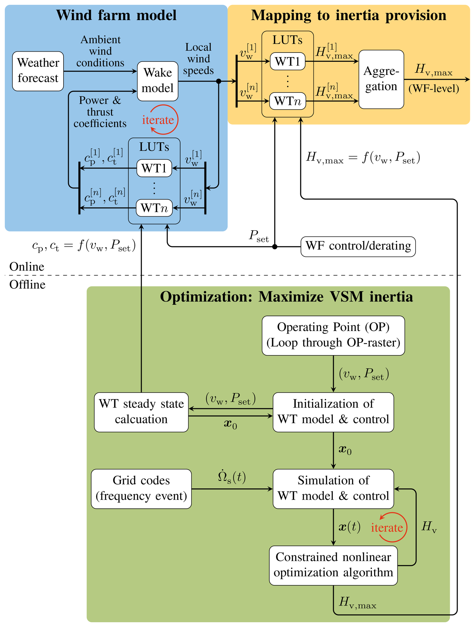
Figure 1 Overview of the proposed WF inertia forecasting approach, which predicts the maximum deliverable inertia constant $H_{\mathrm{v},max}$ of the WF based on online weather forecasting and offline-calculated LUTs.

LUTs of the form $H_{\mathrm{v},max}=f(v_{\mathrm{w}},P_{\text{set}})$ are calculated offline in Fig. 1 by solving optimization problems, which maximize the VSM inertia constant H_v for a given WT operating point (v_w,P_set) and a reference frequency event defined by grid codes. More precisely, an optimization algorithm iteratively runs simulations of the WT response to a ROCOF ${\dot{\mathrm{\Omega }}}_{\mathrm{s}}\left(t\right)$ with different H_v to find the maximum VSM inertia constant $H_{\mathrm{v},max}$ that the WT can provide without violating operating constraints. With the frequency event starting at t=t₀, the operating constraints ensure that the WT states x(t) are within their admissible value range for all t≥t₀. The LUTs $H_{\mathrm{v},max}=f(v_{\mathrm{w}},P_{\text{set}})$ are evaluated online in Fig. 1 to map the WT operating points to the maximum inertia constants $H_{\mathrm{v},max}^{\left[\mathrm{1}\right]},\mathrm{\dots },H_{\mathrm{v},max}^{\left[n\right]}$ of all n WTs. Finally, assuming an optimal $H_{\mathrm{v}}=H_{\mathrm{v},max}$ tuning for each WT in the WF and aggregating $H_{\mathrm{v},max}^{\left[\mathrm{1}\right]},\mathrm{\dots },H_{\mathrm{v},max}^{\left[n\right]}$ yield the inertia provision in terms of the maximum inertia constant $H_{\mathrm{v},max}$ at WF level. The proposed approach is generic because it is applicable to different modeling and control formulations of WTs and WFs.

Although wake effects are taken into account for the initial conditions, the proposed approach assumes that the wind conditions do not change for the duration Δt of the frequency event. Despite the volatile nature of real wind profiles, such an assumption for inertia forecasting at the WF level is reasonable because of an expected averaging effect of any local fluctuations due to the aggregation over several WTs. Moreover, the change in turbine waking during the inertial response is typically negligible due to the propagation delay of farm flow effects. For example, consider a moderate-sized onshore WT with a rated wind speed of 10 m s⁻¹ and a rotor diameter of 130 m. In onshore farms, WTs are usually spaced between 2 D and 5 D from each other in an optimal layout design subject to spacing constraints (Stanley et al., 2022). For the worst-case scenario of a very short 2 D spacing, any change in control action on the upstream WT will take ca. 26 s to reach the downstream WT. This time duration is much greater than the inertial response time or the duration of a severe ROCOF, which lasts only a few seconds.

3.1 Ambient WF wind forecast

Wind conditions are forecasted using fully connected neural networks (FCNNs) based on the methods discussed in Anand et al. (2024). The training targets are the north-aligned component $v_{\mathrm{w}}^u$ and the east-aligned component $v_{\mathrm{w}}^v$ of the wind measurements at the site over the forecast horizon. Wind speed and direction measurements are obtained from historical SCADA data; this way, the coarse-resolution predictions of numerical weather prediction (NWP) models are brought to the specific site where the WF is located. Features from the two NWP models ICON-EU and ARPEGE are used as input data (Zängl et al., 2015; Courtier et al., 1991), together with the u and v components at the present and previous timestamps. The choice of forecast horizon may range from several minutes to several hours, depending on the application use case. For example, for a short-term availability prediction, a forecast horizon of a few minutes to 1 h is relevant. However, a forecast horizon of up to 36 h can be necessary for energy market applications.

The probabilistic wind forecast is obtained using a machine-learning-based model that utilizes Gaussian mixture distributions formed by superimposing several normal distributions. The resulting probability distribution is given by

$$\begin{array}{}\text{(2)}& p\left(x\right)=\sum _i^n{w}_{i}N\left(x\right|{\mathit{\mu }}_i,{\mathit{\sigma }}_i),\end{array}$$

where w_i represents the weight, μ_i the mean, and σ_i the standard deviation of the ith Gaussian normal distribution. Due to the long forecast horizon, an ensemble method consisting of several FCNNs was utilized to predict the parameters w_i, μ_i, and σ_i, where each network is trained only on a specific segment of the overall forecast horizon. This approach was chosen due to its ability to deliver an improved forecast accuracy for each individual segment, as opposed to using networks designed to forecast over the entire time horizon. By focusing on shorter segments, the model can better capture dynamic variations and nuances in the data, leading to more precise predictions. The final forecast is obtained by combining the outputs from multiple ensemble networks, each trained on a specific segment of the data. This ensemble method enhances the overall reliability and accuracy of the forecast. In particular, using a configuration with four networks proved to be an effective compromise, striking a balance between maintaining robustness and minimizing the training time required. This formulation allows for sufficient model flexibility while optimizing computational efficiency, making it a practical choice for operational forecasting.

To reduce the number of input parameters for the FCNNs, a feature-selection algorithm is applied to each of the FCNNs within the ensemble. This is followed by a hyper-parameter optimization process to determine an appropriate number n of normal distributions for the mixed distribution, and to fine-tune both the individual FCNN architectures and the training optimizer. The hyper-parameter optimization is automated and utilizes policy gradients with parameter-based exploration (PGPE) (Sehnke et al., 2010). The training process employs the Adam optimizer, using a mean squared error loss function (Kingma and Ba, 2014). The dataset is divided into training (88 %) and validation (12 %) subsets.

3.2 Local WT operating point prediction

A steady-state engineering flow model is employed to predict the local inflow conditions at each WT within the WF (NREL, 2022). The flow model takes ambient weather forecasts as inputs and models the path and flow characteristics of all wakes within the WF, for given turbine characteristics and operational setpoints. Offline-computed WT LUTs of the form c_p, $c_{\mathrm{t}}=f(v_{\mathrm{w}},P_{\text{set}})$ map the local wind speed v_w and power setpoint P_set to the power coefficient c_p and thrust coefficient c_t. In general, the flow speed v_w at a downstream WT depends on the c_t of the upstream WTs. Thus, the wake model iteratively computes the local wind speeds at all WTs, as shown in Fig. 1.

3.3 WT modeling and control

Figure 2 depicts the overall WT modeling and control used in this work. During normal operation, the MRS-based power setpoint ${\stackrel{\mathrm{‾}}{P}}_{\text{set}}^{\star }$ defines the electromagnetic torque M_e in per unit (p.u.) of rated torque m_R (at the low-speed shaft in N m). During frequency events, M_e additionally depends on the active power droop and inertia provision through VSM control. Details of these torque controllers follow in Sect. 3.3.2–3.3.5.

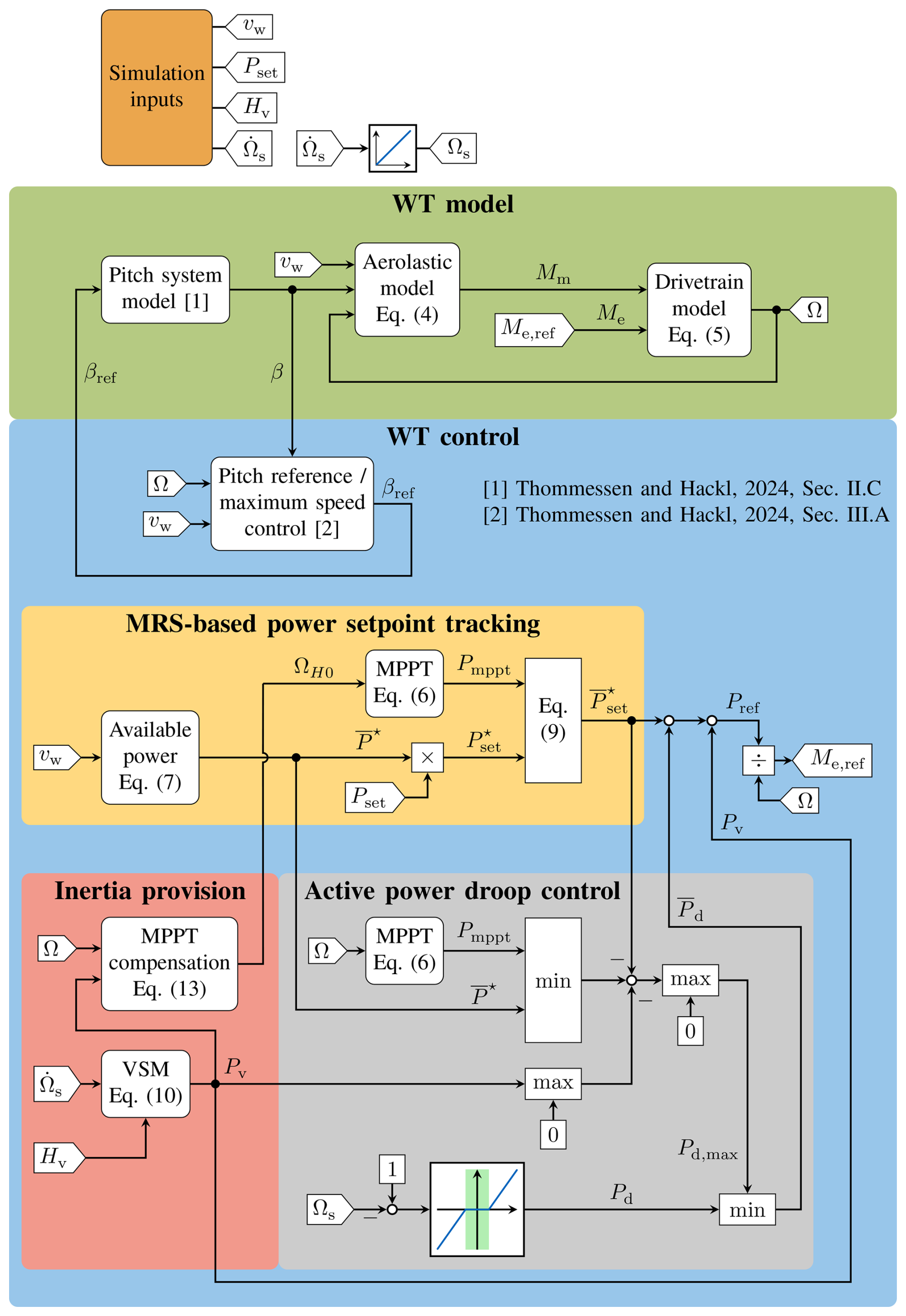
Figure 2 WT modeling and control for solving the optimization problem in Eq. (14). The simplified control representation for the iterative simulations during optimization is derived based on the VSM control for WTs in Thommessen and Hackl (2024). All saturations or manipulations of the power reference P_ref for WT protection have been removed and converted into corresponding optimization constraints.

A standard pitch control strategy is assumed, with the main objective to limit the WT rotor speed Ω, expressed in per unit of rated WT rotor speed ω_R, by adjusting the blade pitch angle β. More precisely, the pitch controller, implemented based on Thommessen and Hackl (2024, Sect. III.A), increases the blade pitch angle reference β_ref for above-rated wind speeds to limit the rotor speed to Ω=1. In addition to Ω, the wind speed v_w is also required as input for the pitch control in Fig. 2 in order to adapt the lower pitch angle limit β_min based on the tip speed ratio $\mathit{\lambda }\propto {v_{\mathrm{w}}}^{-\mathrm{1}}$; i.e., ${\mathit{\beta }}_{\text{ref}}\ge {\mathit{\beta }}_{min}\left(\mathit{\lambda }\right)$. This is more relevant for derating than for MPPT.

The WT physical inertia constant H (which should rather be called “inertia variable” due to the variable Ω) is proportional to the WT kinetic energy E_kin; i.e.,

$$\begin{array}{}\text{(3)}& H:={\displaystyle \frac{E_{\text{kin}}}{p_{\mathrm{R}}}}:={\displaystyle \frac{\frac{\mathrm{1}}{\mathrm{2}}\mathrm{\Theta }{\mathit{\omega }}^{\mathrm{2}}}{p_{\mathrm{R}}}}={\mathrm{\Omega }}^{\mathrm{2}}{H}_{\mathrm{R}},\end{array}$$

where H_R denotes the inertia constant at rated speed Ω=1. Note that, for (directly grid-connected) SMs (of conventional power plants), it follows that $H={{\mathrm{\Omega }}_{\mathrm{s}}}^{\mathrm{2}}{H}_{\mathrm{R}}\approx H_{\mathrm{R}}$ due to an approximately constant SM rotor speed or system frequency Ω_s≈1.

3.3.1 Aeroelastic and mechanical model

The power coefficient c_p and the thrust coefficient c_t are modeled as functions of tip speed ratio λ and blade pitch angle β by the corresponding LUTs. The fore–aft deflection of the WT tower, excited by the thrust force F_t, is modeled as a mass–spring–damper oscillator with mass m_t, damping coefficient d_t, and stiffness coefficient k_t. The aeroelastic model outputs the WT mechanical torque M_m (in p.u. of m_R) for given inputs $(v_{\mathrm{w}},\mathit{\beta },\mathrm{\Omega })$; i.e.,

$$\begin{array}{}\text{(4a)}& {\displaystyle }{P}_{\mathrm{w}}={\displaystyle \frac{\mathrm{1}}{\mathrm{2}}}\mathit{\rho }\mathit{\pi }{r}^{\mathrm{2}}{v_{\mathrm{w}}}^{\mathrm{3}}/p_{\mathrm{R}},\text{(4b)}& {\displaystyle }{M}_{\mathrm{m}}={\displaystyle \frac{P_{\mathrm{m}}}{\mathrm{\Omega }}}={\displaystyle \frac{P_{\mathrm{w}}{c}_{\mathrm{p}}(\mathit{\lambda },\mathit{\beta })}{\mathrm{\Omega }}},\mathit{\lambda }=\mathrm{\Omega }{\displaystyle \frac{{\mathit{\omega }}_{\mathrm{R}}r}{{\stackrel{\mathrm{̃}}{v}}_{\mathrm{w}}}},{\stackrel{\mathrm{̃}}{v}}_{\mathrm{w}}=v_{\mathrm{w}}-{\dot{s}}_{\mathrm{t}},\text{(4c)}& {\displaystyle }\begin{array}{rl}& {\ddot{s}}_{\mathrm{t}}={\displaystyle \frac{\mathrm{1}}{m_{\mathrm{t}}}}\left(F_{\mathrm{t}}-d_{\mathrm{t}}{\dot{s}}_{\mathrm{t}}-k_{\mathrm{t}}{s}_{\mathrm{t}}\right),F_{\mathrm{t}}={\displaystyle \frac{\mathrm{1}}{\mathrm{2}}}\mathit{\rho }\mathit{\pi }{r}^{\mathrm{2}}{v}_{\mathrm{w}}^{\mathrm{2}}{c}_{\mathrm{t}}(\mathit{\lambda },\mathit{\beta }),\\ & s_{\mathrm{t},\mathrm{0}}={\displaystyle \frac{F_{\mathrm{t}}}{k_{\mathrm{t}}}},{\dot{s}}_{\mathrm{t},\mathrm{0}}=\mathrm{0},\end{array}\end{array}$$

with wind power P_w (in p.u. of p_R); WT aerodynamic or mechanical power P_m (in p.u. of p_R); air density ρ; rotor radius r; relative wind speed ${\stackrel{\mathrm{̃}}{v}}_{\mathrm{w}}$; WT fore–aft tower displacement s_t; and initial steady-state values $s_{\mathrm{t},\mathrm{0}},{\dot{s}}_{\mathrm{t},\mathrm{0}},{\mathit{\lambda }}_{\mathrm{0}}$, and β₀. Using H_R (in s) to indicate the WT total physical drivetrain inertia constant, the WT mechanical dynamics are approximated by a one-mass model (Thommessen and Hackl, 2024); i.e.,

$$\begin{array}{}\text{(5)}& \dot{\mathrm{\Omega }}={\displaystyle \frac{M_{\mathrm{m}}-M_{\mathrm{e}}}{\mathrm{2}{H}_{\mathrm{R}}}},\mathrm{\Omega }\left(\mathrm{0}\right)={\mathrm{\Omega }}_{\mathrm{0}}.\end{array}$$

3.3.2 Maximum rotation strategy

The electrical power for MPPT is given by

$$\begin{array}{}\text{(6)}& P_{\text{mppt}}:=\mathrm{\Omega }{M}_{\text{mppt}},\end{array}$$

where the MPPT torque is the function of rotor speed M_mppt:=M_mppt(Ω), shown in Fig. 3.

Figure 3 MPPT torque as a function of rotor speed Ω.

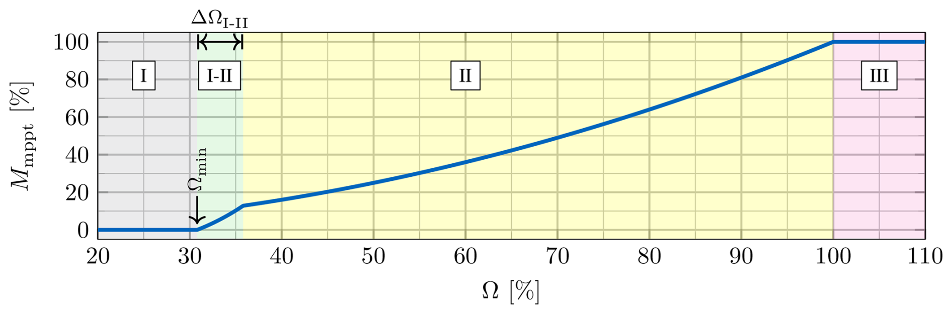
Below rated wind speed in region II, M_mppt increases proportionally to Ω² for optimal operation at the MPP. Above rated wind speed in region III, the pitch control limits the WT rotor speed to Ω=1 such that $P_{\text{mppt}}=M_{\text{mppt}}=\mathrm{1}$. Below cut-in wind speed v_w,cut-in in region I, the WT does not generate power; i.e., M_mppt=0 for $\mathrm{\Omega }<{\mathrm{\Omega }}_{min}$. For a smooth transition to region II, a non-optimal operation is accepted in the small transition region I–II, defined by ${\mathrm{\Omega }}_{min}\le \mathrm{\Omega }\le {\mathrm{\Omega }}_{min}+\mathrm{\Delta }{\mathrm{\Omega }}_{\text{I-II}}$; i.e., M_mppt is obtained by multiplying the optimal torque at the MPP by a factor that is linearly interpolated between 0 at Ω_min and 1 at ${\mathrm{\Omega }}_{min}+\mathrm{\Delta }{\mathrm{\Omega }}_{\text{I-II}}$. For a more complete description of the MPPT curve, see Thommessen and Hackl (2024, Sect. III.B.1).

The MRS-based derating maximizes the WT kinetic energy reserve for inertia provision. The derating power setpoint P_set is defined relative to the MPP; i.e., P_set=1 corresponds to MPPT, and P_set<1 corresponds to derating. Increasing derating (decreasing P_set) reduces the electrical power setpoint $P_{\text{set}}^{\star }:={\stackrel{\mathrm{‾}}{P}}^{\star }{P}_{\text{set}}$ with available power ${\stackrel{\mathrm{‾}}{P}}^{\star }\in (\mathrm{0},\mathrm{1}]$; i.e., the WT accelerates. As a consequence, the tip speed ratio λ increases, and the power coefficient c_p decreases. The pitch controller additionally increases β if necessary to limit the rotor speed to Ω=1. In general, the MRS prioritizes increasing WT speed over pitching to provide power reserve.

With the measured or estimated rotor-effective wind speed v_w (Soltani et al., 2013), the available power in Fig. 2 is defined as

$$\begin{array}{}\text{(7)}& {\stackrel{\mathrm{‾}}{P}}^{\star }:=P_{\mathrm{w}}\left(v_{\mathrm{w}}\right){\stackrel{\mathrm{‾}}{c}}_{\mathrm{p}}^{\star }\left(v_{\mathrm{w}}\right):={\displaystyle \frac{\mathrm{1}}{\mathrm{2}}}\mathit{\rho }\mathit{\pi }{r}^{\mathrm{2}}{v_{\mathrm{w}}}^{\mathrm{3}}{\stackrel{\mathrm{‾}}{c}}_{\mathrm{p}}^{\star }\left(v_{\mathrm{w}}\right)/p_{\mathrm{R}},\end{array}$$

where the MPPT (P_set=1) power coefficient is given by

$$\begin{array}{}\text{(8)}& {\stackrel{\mathrm{‾}}{c}}_{\mathrm{p}}^{\star }\left(v_{\mathrm{w}}\right)=\left\{\begin{array}{ll}{c}_{\mathrm{p}}({\stackrel{\mathrm{‾}}{\mathrm{\Omega }}}^{\star },{\stackrel{\mathrm{‾}}{\mathit{\beta }}}^{\star },v_{\mathrm{w}})& \text{if}{v}_{\mathrm{w},\text{cut-in}}\le v_{\mathrm{w}}<v_{\mathrm{w},\text{II},min},\\ & \\ c_{\mathrm{p}}^{\star }:=max{c}_{\mathrm{p}}& \text{if}{v}_{\mathrm{w},\text{II},min}\le v_{\mathrm{w}}\le v_{\mathrm{w},\mathrm{R}},\\ & \\ \frac{\mathrm{1}}{P_{\mathrm{w}}\left(v_{\mathrm{w}}\right)}& \text{if}{v}_{\mathrm{w},\mathrm{R}}<v_{\mathrm{w}}\le v_{\mathrm{w},\text{cut-out}},\end{array}\right.\end{array}$$

with cut-in wind speed v_w,cut-in, minimum region-II wind speed v_w,II, rated wind speed v_w,R, cut-out wind speed v_w,cut-out, and steady-state values $({\stackrel{\mathrm{‾}}{\mathrm{\Omega }}}^{\star },{\stackrel{\mathrm{‾}}{\mathit{\beta }}}^{\star })$.

Limiting $P_{\text{set}}^{\star }$ by P_mppt for rotor speed transients and wind measurement errors, the saturated power setpoint is given by

$$\begin{array}{}\text{(9)}& \begin{array}{rl}{\stackrel{\mathrm{‾}}{P}}_{\text{set}}^{\star }& :=\left\{\begin{array}{ll}min(P_{\text{set}}^{\star },P_{\text{mppt}}),& \text{if}{P}_{\text{set}}<\mathrm{1}\left(\text{derating}\right),\\ P_{\text{mppt}},& \text{if}{P}_{\text{set}}=\mathrm{1}\left(\text{MPPT}\right).\end{array}\right\}\\ & \text{with}{P}_{\text{set}}^{\star }:={\stackrel{\mathrm{‾}}{P}}^{\star }{P}_{\text{set}}.\end{array}\end{array}$$

$P_{\text{set}}^{\star }$ is ignored for P_set=1 (MPPT) in Eq. (9), since (i) no wind measurements are required, and (ii) smaller transient rotor speed overshoots occur due to higher power setpoint adaptation. For example, if Ω>1 due to a wind gust, it follows that ${\stackrel{\mathrm{‾}}{P}}_{\text{set}}^{\star }=P_{\text{mppt}}=\mathrm{\Omega }{M}_{\text{mppt}}>\mathrm{1}$, whereas $P_{\text{set}}^{\star }\le \mathrm{1}$.

3.3.3 VSM control

Grid-forming control is required to limit the initial ROCOF (ESIG, 2022; VDE, 2024a). This paper simplifies the grid-forming VSM control proposed in Thommessen and Hackl (2024) by neglecting fast electromagnetic transients and low-level current control loops. However, the grid synchronization dynamics of grid-forming control define the inertial response and must therefore be taken into account.

For VSM control, the grid synchronization dynamics are similar to the dynamics of a real (grid-connected) SM, as illustrated in Fig. 4.

Figure 4 Grid synchronization loop of a freely spinning VSM.

The VSM acceleration ${\dot{\mathrm{\Omega }}}_{\mathrm{v}}$ is proportional to the sum of virtual torques; i.e., the VSM mechanical model is based on a one-mass model with virtual inertia H_v instead of physical inertia H_R in Eq. (5). At steady state, the difference between VSM mechanical and electromagnetic torque is zero (i.e., $M_{\mathrm{m},\mathrm{v}}-M_{\mathrm{e},\mathrm{v}}=\mathrm{0}$), and the VSM damping torque is zero (i.e., $M_{\text{dp},\mathrm{v}}=\mathrm{0}$). Since only the inertial response to ROCOFs or electromagnetic changes is of interest, the VSM mechanical torque is set to zero (i.e., $M_{\mathrm{m},\mathrm{v}}=\mathrm{0}$), resulting in the freely spinning VSM in Fig. 4. Denormalization of the power system frequency, i.e., ${\mathit{\omega }}_{\mathrm{s}}={\mathrm{\Omega }}_{\mathrm{s}}{\mathit{\omega }}_{\mathrm{s},\mathrm{R}}$ with ${\mathit{\omega }}_{\mathrm{s},\mathrm{R}}:=\mathrm{2}\mathit{\pi }{f}_{\mathrm{s},\mathrm{R}}$, and subsequent integration of ω_s yield the grid or system angle ϕ_s. Similarly, denormalization of the VSM rotor speed, i.e., ${\mathit{\omega }}_{\mathrm{v}}={\mathrm{\Omega }}_{\mathrm{v}}{\mathit{\omega }}_{\mathrm{s},\mathrm{R}}$, and subsequent integration of ω_v yield the VSM rotor angle ϕ_v. The VSM electromagnetic torque M_e,v depends on the (real) load angle $\mathit{\delta }:={\mathit{\varphi }}_{\mathrm{v}}-{\mathit{\varphi }}_{\mathrm{s}}$ multiplied by the electromagnetic feedback gain k_e. Due to unknown ϕ_s or k_e, the VSM controller calculates the torque or power feedback directly based on current and grid voltage measurements. The VSM damping torque M_dp,v is proportional to the VSM slip Ω_v−Ω_s, which emulates the effect of damper windings in SMs. However, unlike real SMs, the VSM enables flexible tuning of the VSM damping D_v. Grid voltage measurements are required to determine Ω_s for VSM damping torque calculation.

The VSM power for inertia provision, added to the power setpoint ${\stackrel{\mathrm{‾}}{P}}_{\text{set}}^{\star }$ in Fig. 2, is defined as

$$\begin{array}{}\text{(10)}& P_{\mathrm{v}}={\mathrm{\Omega }}_{\mathrm{v}}{M}_{\mathrm{e},\mathrm{v}},\end{array}$$

where Ω_v and M_e,v are given by the grid synchronization loop in Fig. 4 with input ${\dot{\mathrm{\Omega }}}_{\mathrm{s}}$.

The inertial response in the Laplace domain of the VSM is given by (Thommessen and Hackl, 2024)

$$\begin{array}{}\text{(11)}& \begin{array}{rl}& {\displaystyle \frac{M_{\mathrm{e},\mathrm{v}}}{{\dot{\mathrm{\Omega }}}_{\mathrm{s}}}}={\displaystyle \frac{-k_{\mathrm{e}}{\mathit{\omega }}_{\mathrm{s},\mathrm{R}}}{s^{\mathrm{2}}+\mathrm{2}{\mathit{\zeta }}_{\mathrm{v}}{\mathit{\omega }}_{\mathrm{n},\mathrm{v}}s+{\mathit{\omega }}_{\mathrm{n},\mathrm{v}}^{\mathrm{2}}}},{\mathit{\omega }}_{\mathrm{n},\mathrm{v}}^{\mathrm{2}}:={\displaystyle \frac{k_{\mathrm{e}}{\mathit{\omega }}_{\mathrm{s},\mathrm{R}}}{\mathrm{2}{H}_{\mathrm{v}}}},\\ & {\mathit{\zeta }}_{\mathrm{v}}:={\displaystyle \frac{D_{\mathrm{v}}}{\sqrt{\mathrm{8}{H}_{\mathrm{v}}{k}_{\mathrm{e}}{\mathit{\omega }}_{\mathrm{s},\mathrm{R}}}}}=\mathrm{1}\Rightarrow D_{\mathrm{v}}:=D_{\mathrm{v}}\left(H_{\mathrm{v}}\right):=\sqrt{\mathrm{8}{H}_{\mathrm{v}}{k}_{\mathrm{e}}{\mathit{\omega }}_{\mathrm{s},\mathrm{R}}},\end{array}\end{array}$$

with natural angular velocity ω_n,v and damping ratio chosen as ζ_v=1 to avoid overshooting. With grid-synchronized VSM speed ${\mathrm{\Omega }}_{\mathrm{v}}={\mathrm{\Omega }}_{\mathrm{s}}\approx \mathrm{1}$ in Eq. (10) and setting s=0 in Eq. (11), the steady-state VSM power for a constant ROCOF simplifies to

$$\begin{array}{}\text{(12)}& P_{\mathrm{v}}={\mathrm{\Omega }}_{\mathrm{v}}{M}_{\mathrm{e},\mathrm{v}}\approx M_{\mathrm{e},\mathrm{v}}\approx -\mathrm{2}{H}_{\mathrm{v}}{\dot{\mathrm{\Omega }}}_{\mathrm{s}}.\end{array}$$

The power system dynamics in Fig. 4 are defined by a reference frequency event. The electromagnetic feedback in Fig. 4 depends on the load angle given by the angle difference between the VSM and the grid; i.e., $M_{\mathrm{e},\mathrm{v}}=k_{\mathrm{e}}\mathit{\delta }=k_{\mathrm{e}}\left({\mathit{\varphi }}_{\mathrm{v}}-{\mathit{\varphi }}_{\mathrm{s}}\right)$. For simplicity, this paper assumes a constant electromagnetic feedback gain k_e. Actually, k_e depends on the WT operating point and the WT grid connection; i.e., k_e is a nonlinear function of the load angle delta δ, the grid voltage, and the grid impedance (VDE, 2024a; Ghimire et al., 2025). Type 3 WTs use doubly fed induction machines (DFIMs), where k_e also depends on the DFIM rotor current or excitation level (Thommessen and Hackl, 2024, Sect. III.E). If not negligible, the dependency of k_e on δ and the excitation level should be taken into account based on the WT operating point. With admissible limits for grid voltage and impedance defined by grid codes (VDE, 2024a), k_e should be chosen based on the WT grid connection, as explained in Appendix B.

This paper assumes internal damping of the VSM (Roscoe et al., 2020; Thommessen and Hackl, 2024); i.e., the damping torque M_dp,v in Fig. 4 is solely virtual and is not converted into real electrical output power. In contrast, for external damping of a real SM, the damping power is part of the electrical output power (Roscoe et al., 2020). In this regard, H_v of a VSM and H of a (real) SM differ; i.e., assuming H_v=H and equal damping gains, the actually extracted kinetic energy during the inertial response is smaller for a VSM-controlled WT than for a (real) SM.

Figure 5 shows an exemplary inertial power response to a ROCOF with quasi-steady-state amplitude ΔP approximated by Eq. (12).

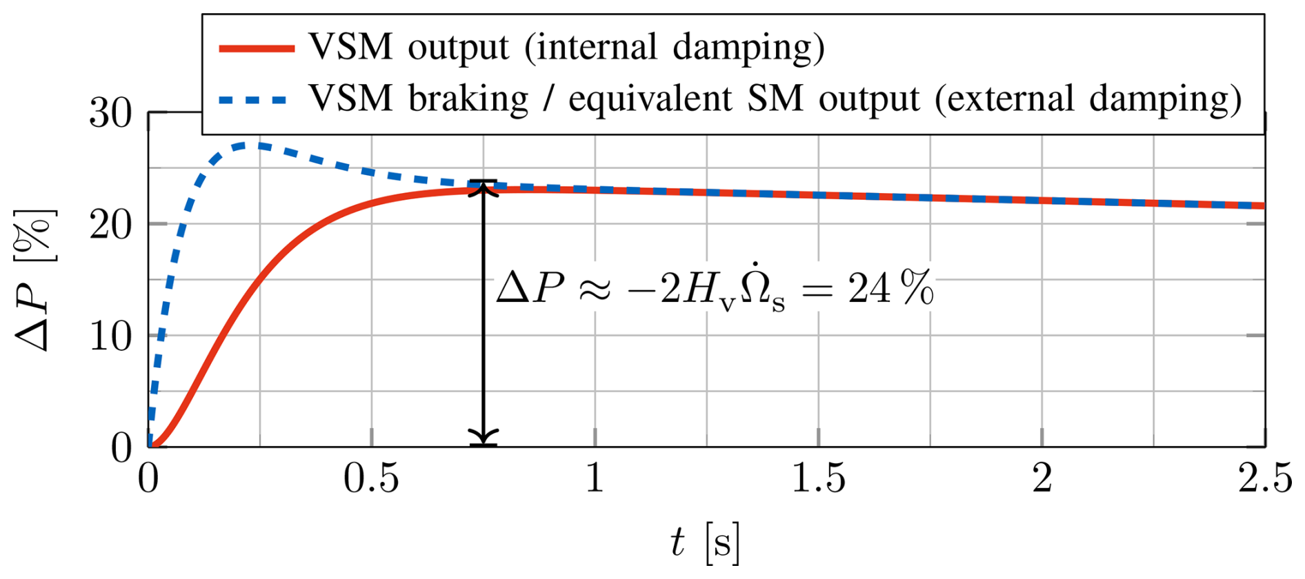
Figure 5 Inertial power response to a ROCOF of ${\dot{\mathrm{\Omega }}}_{\mathrm{s}}=-\mathrm{4}\mathrm{\%}{\mathrm{s}}^{-\mathrm{1}}$ for H_v=3 s with quasi-steady-state amplitude ΔP approximated by Eq. (12). The VSM achieves the desired internal damping of the VSM output power, whereas the VSM braking power overshoots. The VSM output power equals the WT electrical power change. The VSM braking power equals the electrical power of an equivalent real SM with external damping; i.e., the SM braking energy is fully converted into electrical energy according to the law of conservation of energy.

The damping energy corresponds to the area between the two curves in Fig. 5. Strictly speaking, the VSM concept violates the law of conservation of energy since the VSM braking energy is not fully converted into electrical energy. However, high internal damping avoids power overshoots and is beneficial for grid frequency stability (Roscoe et al., 2020; Thommessen and Hackl, 2024). Also, grid codes require sufficient damping and consider (internal) damping power separately from electrical output power (VDE, 2024a, Kap. 5.1.1.11, Anmerkung 1). Finally, H_v is comparable to H of a real SM when neglecting the transient damping, i.e., when considering the quasi-steady-state power change $\mathrm{\Delta }P=-\mathrm{2}{H}_{\mathrm{v}}{\dot{\mathrm{\Omega }}}_{\mathrm{s}}$, as shown in Fig. 5. Thus, H_v is a suitable measure for the inertial power response and the grid frequency support by inertia provision.

The recent draft VDE (2024b) for certification of grid-forming IBRs quantifies inertia provision by the mean power change over a time window starting 0.5 s after a ROCOF change and ending at the beginning of the next ROCOF change during the reference frequency event; i.e., $T_{\mathrm{A}}:=\text{mean}\left|\mathrm{\Delta }P\right(t)/{\dot{\mathrm{\Omega }}}_{\mathrm{s}}|\approx \mathrm{2}{H}_{\mathrm{v}}$. For example, due to a constant initial ROCOF for 1 s during the reference frequency event starting at t=0, the first time window for quantifying inertia provision is $\mathrm{0.5}\mathrm{s}\le t\le \mathrm{1}\mathrm{s}$. For simplicity, this paper quantifies inertia provision by the control parameter H_v (see also Fig. 5), which results in a (slight) overestimation of the inertia provision compared to VDE (2024b).

This paper assumes an ideal inertial power response; i.e., the VSM power P_v is added to the original machine power setpoint ${\stackrel{\mathrm{‾}}{P}}_{\text{set}}^{\star }$ in Fig. 2. Moreover, the final electromagnetic torque equals the electromagnetic torque reference, i.e., $M_{\mathrm{e}}=M_{\mathrm{e},\text{ref}}$ in Fig. 2, neglecting low-level current controls with closed-loop time constants that are significantly smaller than the ones of high-level WT or VSM control. Clearly, this is a simplified representation of the actual VSM control, which adjusts the voltage or current phase angle based on the VSM angle ϕ_v to achieve the grid-forming capability (ESIG, 2022; Thommessen and Hackl, 2024). Although the implementation details are beyond the scope of this paper, the simplified representation should take into account the general differences between existing VSM control strategies, as discussed in Appendices C–E.

3.3.4 MPPT compensation

For a negative ROCOF, the WT output power increases for inertia provision, which decelerates the WT. According to Eq. (6), the MPPT would counteract the deceleration by reducing P_mppt when Ω decreases. To avoid this, the so-called MPPT compensation manipulates the MPPT input Ω (Duckwitz, 2019; Thommessen and Hackl, 2024). This paper simplifies the MPPT compensation proposed in Thommessen and Hackl (2024, Sect. III.B.2). The speed change due to inertia provision is estimated by replacing the numerator of the one-mass model in Eq. (5) by the inertial torque change $P_{\mathrm{v}}/\mathrm{\Omega }$. Thus, the manipulated MPPT input, equal to the theoretical WT rotor speed for zero inertia provision, is given by

$$\begin{array}{}\text{(13)}& \begin{array}{rl}& {\mathrm{\Omega }}_{H\mathrm{0}}:=\mathrm{\Omega }+\left\{\begin{array}{l}min\left\{a,\frac{\mathrm{1}}{\mathrm{2}{H}_{\mathrm{R}}}{\int }_{t_{\mathrm{0}}}^t\frac{P_{\mathrm{v}}}{\mathrm{\Omega }}\mathrm{d}t\right\},\\ \text{if}\left|{\dot{\mathrm{\Omega }}}_{\mathrm{v}}\right|>\mathit{ϵ}\left(\text{active MPPT comp.}\right),\\ \mathrm{0},\\ \text{if}\left|{\dot{\mathrm{\Omega }}}_{\mathrm{v}}\right|\le \mathit{ϵ}\left(\text{inactive MPPT comp.}\right),\end{array}\right\},\\ & a:=max\left\{\mathrm{1}-\mathrm{\Omega },\mathrm{0}\right\},\end{array}\end{array}$$

with the threshold ϵ used for detecting active inertia provision based on the VSM acceleration ${\dot{\mathrm{\Omega }}}_{\mathrm{v}}\approx {\dot{\mathrm{\Omega }}}_{\mathrm{s}}$. The integral in Eq. (13) is reset to zero for inactive MPPT compensation. The actual implementation of Eq. (13) includes an additional rate limiter, which ensures $\left|{\dot{\mathrm{\Omega }}}_{H\mathrm{0}}\right|\le {\dot{\mathrm{\Omega }}}_{H\mathrm{0},max}$ with maximum acceleration ${\dot{\mathrm{\Omega }}}_{H\mathrm{0},max}$ for a smooth transition between active and inactive MPPT compensation (Thommessen and Hackl, 2024, Sect. III.B.2).

Assuming active MPPT compensation, a prolonged MPP deviation during a long time period with a small negative ROCOF would lead to excessive WT rotor deceleration. Thus, the threshold ϵ in Eq. (13) should not be chosen too small. This also implies less inertia provision for small negative ROCOFs $\left|{\dot{\mathrm{\Omega }}}_{\mathrm{s}}\right|\approx \left|{\dot{\mathrm{\Omega }}}_{\mathrm{v}}\right|\le \mathit{ϵ}$ than expected by H_v due to the MPPT compensation being inactive. Also, for $\mathit{ϵ}<\left|{\dot{\mathrm{\Omega }}}_{\mathrm{s}}\right|<{\dot{\mathrm{\Omega }}}_{\mathrm{s},max}$ with normalized worst-case ROCOF magnitude ${\dot{\mathrm{\Omega }}}_{\mathrm{s},max}$, there may be cases when the inertia provision is (slightly) smaller than expected by H_v, if output power saturation is required to protect the rotor speed due to prolonged MPP deviations. However, the proposed approach ensures unsaturated or full inertia provision when reaching the worst-case or reference ROCOF $\left|{\dot{\mathrm{\Omega }}}_{\mathrm{s}}\right|={\dot{\mathrm{\Omega }}}_{\mathrm{s},max}$.

3.3.5 Active power droop control

In addition to inertia provision, which supports grid frequency by injecting inertial VSM power P_v proportional to the ROCOF, active power droop control supports grid frequency by injecting (saturated) droop power ${\stackrel{\mathrm{‾}}{P}}_{\mathrm{d}}$ proportional to the frequency deviation $\mathrm{\Delta }{\mathrm{\Omega }}_{\mathrm{s}}:=\mathrm{1}-{\mathrm{\Omega }}_{\mathrm{s}}$. Thus, the final power reference in Fig. 2 is given by $P_{\text{ref}}={\stackrel{\mathrm{‾}}{P}}_{\text{set}}^{\star }+P_{\mathrm{v}}+{\stackrel{\mathrm{‾}}{P}}_{\mathrm{d}}$. For WTs, droop control is inactive during normal operation within a tolerance band of $\left|\mathrm{\Delta }{\mathrm{\Omega }}_{\mathrm{s}}\right|\le \mathrm{0.4}\mathit{\%}$ (VDE, 2024a); i.e., the (unsaturated) droop power is $P_{\mathrm{d}}={\stackrel{\mathrm{‾}}{P}}_{\mathrm{d}}=\mathrm{0}$ in Fig. 2. During a critical system state outside of the tolerance band, the WTs have to support grid frequency by a proportional power adaptation when possible. This means that ${\stackrel{\mathrm{‾}}{P}}_{\mathrm{d}}=P_{\mathrm{d}}>\mathrm{0}$ is only required if wind power reserves are available due to previous derating (VDE, 2024a). For the present control strategy, this implies that the inertia provision based on additional kinetic energy extraction is prioritized over droop control; see Appendix F for details.

Ignoring the two max blocks in Fig. 2, the maximum droop power $P_{\mathrm{d},max}$ is given by the total currently available power $min({\stackrel{\mathrm{‾}}{P}}^{\star },P_{\text{mppt}})$ minus the sum of the power setpoint ${\stackrel{\mathrm{‾}}{P}}_{\text{set}}^{\star }$ and the VSM power P_v. The saturation ${\stackrel{\mathrm{‾}}{P}}_{\mathrm{d}}:=min(P_{\mathrm{d}},P_{\mathrm{d},max})$ prevents excessive WT overloading since, without it, the droop power P_d would add to the inertial power even if the output or reference power P_ref already exceeds the available one. In other words, the WT control prioritizes inertia provision over droop control. Similarly, for real (grid-connected) SMs, the droop control or speed governor response time is significantly slower than the SM inertial response; i.e., only the SM inertial power limits the initial ROCOF.

The additional saturations by the two max blocks in Fig. 2 ensure that the droop control power P_d does not counteract the VSM power P_v for inertia provision. Without the upper max block, $P_{\mathrm{d}}=P_{\mathrm{d},max}<\mathrm{0}$ could counteract P_v>0 for a high negative initial ROCOF; without the lower max block, $P_{\mathrm{d}}=P_{\mathrm{d},max}>\mathrm{0}$ could counteract P_v<0 more than expected for a subsequent positive ROCOF during frequency recovery. The presented control is a simplified version of the actual control with dynamic droop saturation of Thommessen and Hackl (2024, Sect. III.F).

3.4 Grid-forming capability of WTs

This section introduces a general approach used for evaluating the grid-forming capability of WTs in terms of maximum inertia provision. First, we present the proposed optimization problem to evaluate the maximum deliverable inertia. Then, we develop two solutions of the problem. The first produces a simplified result derived from the formulations in the existing literature. This is followed by a second complete numerical solution, which utilizes a dynamic model of the WT inertial response within the optimization.

3.4.1 Optimization problem for maximum inertia provision

The maximum feasible VSM inertia constant $H_{\mathrm{v},max}$ is obtained by solving the optimization problem

$$\begin{array}{}\text{(14)}& \begin{array}{rl}& \forall t\ge t_{\mathrm{0}}:H_{\mathrm{v},max}:={\text{arg\hspace{0.17em}max}}_{H_{\mathrm{v}}}\left\{H_{\mathrm{v}}\right\},\\ & \text{s.t.}\left\{\begin{array}{c}\mathrm{\Omega }\left(t\right)\ge {\mathrm{\Omega }}_{min}\\ M_{\mathrm{e}}\left(t\right)\le M_{\mathrm{e},max}\\ {\dot{M}}_{\mathrm{e}}\left(t\right)\le {\dot{M}}_{\mathrm{e},max}\\ P_{\mathrm{e}}\left(t\right)\le P_{\mathrm{e},max}\end{array}\right\}.\end{array}\end{array}$$

Here, the WT electromagnetic torque rate ${\dot{M}}_{\mathrm{e}}:=\frac{\mathrm{d}}{\mathrm{d}t}{M}_{\mathrm{e}}$ is in s⁻¹; the WT electrical power P_e is in p.u. of rated power p_R=ω_Rm_R (in W); and Ω_min, $M_{\mathrm{e},max}$, ${\dot{M}}_{\mathrm{e},max}$, and $P_{\mathrm{e},max}$ denote the admissible operating limits. Note that, although the objective function and optimization argument in Eq. (14) are the same, the solution of this problem is not trivial due to the presence of nonlinear optimization constraints. Depending on the grid codes and WT design, additional constraints may have to be considered, e.g., to account for aerodynamic stall limits (here implicitly taken into account by Ω_min in Eq. 14). Appendix G discusses the case of recovery power limits, with reference to the examples shown later in Sect. 4.

3.4.2 Simplified solution

Lee et al. (2016) evaluate the capability of grid-following WTs to emulate inertia by considering WT rotor speed or available kinetic energy reserve. Here, we depart from that approach by deriving a simplified solution of Eq. (14) for grid-forming WTs that takes all operating constraints into account.

Neglecting any changes in aerodynamic conditions during the inertial response, i.e., assuming constant values for wind speed, pitch angle, and tip speed ratio, it follows that the mechanical power is constant; i.e.,

$$\begin{array}{}\text{(15)}& \begin{array}{rl}\forall t_{\mathrm{0}}& \le t\le t_{\mathrm{0}}+\mathrm{\Delta }t:\left\{\begin{array}{l}{v}_{\mathrm{w}}\left(t\right)=v_{\mathrm{w}}\left(t_{\mathrm{0}}\right)=:v_{\mathrm{w},\mathrm{0}}\\ \mathit{\beta }\left(t\right)=\mathit{\beta }\left(t_{\mathrm{0}}\right)=:{\mathit{\beta }}_{\mathrm{0}}\\ \mathit{\lambda }\left(t\right)=\mathit{\lambda }\left(t_{\mathrm{0}}\right)=:{\mathit{\lambda }}_{\mathrm{0}}\end{array}\right\}\\ & \Rightarrow P_{\mathrm{m}}\left(t\right)=P_{\mathrm{m}}\left(t_{\mathrm{0}}\right)=:P_{\mathrm{m},\mathrm{0}}.\end{array}\end{array}$$

For the simplified solution, we assume that the ROCOF ${\dot{f}}_{\mathrm{s}}$ is constant and equal to the worst-case initial ROCOF, until reaching the minimum frequency nadir $f_{\mathrm{s},min}$ at time $t=t_{\mathrm{s},min}$; i.e., the considered time duration is given by

$$\begin{array}{}\text{(16)}& \mathrm{\Delta }t:=t_{\mathrm{s},min}-t_{\mathrm{0}}={\displaystyle \frac{f_{\mathrm{s},min}-f_{\mathrm{s},\mathrm{R}}}{{\dot{f}}_{\mathrm{s}}}}.\end{array}$$

Assuming that the initial electrical power equals the mechanical power in Eq. (15), i.e., $P_{\mathrm{e},\mathrm{0}}=P_{\mathrm{m},\mathrm{0}}$, and approximating the electrical power change during Δt by an ideal power pulse ΔP_e according to the simplified inertial response in Eq. (1a), the electrical power constraint in Eq. (14) simplifies to

$$\begin{array}{}\text{(17)}& P_{\mathrm{e}}:=P_{\mathrm{e},\mathrm{0}}+\mathrm{\Delta }{P}_{\mathrm{e}}:=P_{\mathrm{m},\mathrm{0}}+\mathrm{2}{H}_{\mathrm{v}}{\dot{\mathrm{\Omega }}}_{\mathrm{s},max}\le P_{\mathrm{e},max},\end{array}$$

where ${\dot{\mathrm{\Omega }}}_{\mathrm{s},max}:=\left|{\dot{f}}_{\mathrm{s},\mathrm{0}}\right|/f_{\mathrm{s},\mathrm{R}}>\mathrm{0}$. It follows that additional output power $\mathrm{\Delta }{P}_{\mathrm{e}}:=\mathrm{2}{H}_{\mathrm{v}}{\dot{\mathrm{\Omega }}}_{\mathrm{s},max}$ is extracted from the WT kinetic energy reserve according to

$$\begin{array}{}\text{(18)}& {\int }_{t_{\mathrm{0}}}^{t_{\mathrm{s},min}}\left(P_{\mathrm{m}}-P_{\mathrm{e}}\right)\mathrm{d}t=E_{\text{kin}}\left(t_{\mathrm{s},min}\right)-E_{\text{kin}}\left(t_{\mathrm{0}}\right),\end{array}$$

from which we get $\mathrm{\Delta }{P}_{\mathrm{e}}\mathrm{\Delta }t=H_{\mathrm{R}}\left({{\mathrm{\Omega }}_{\mathrm{0}}}^{\mathrm{2}}-\mathrm{\Omega }(t_{\mathrm{s},min}{)}^{\mathrm{2}}\right)$. Finally, the minimum rotor speed constraint in Eq. (14) simplifies to

$$\begin{array}{}\text{(19)}& \mathrm{\Omega }\left(t_{\mathrm{s},min}\right)=\sqrt{{{\mathrm{\Omega }}_{\mathrm{0}}}^{\mathrm{2}}-\mathrm{2}{\displaystyle \frac{H_{\mathrm{v}}}{H_{\mathrm{R}}}}\left(\mathrm{1}-{\mathrm{\Omega }}_{\mathrm{s},min}\right)}\ge {\mathrm{\Omega }}_{min},\end{array}$$

where Ω₀:=Ω(t₀), and H_R includes the total inertia of the WT drivetrain. Note that Eq. (19) depends on the normalized frequency nadir ${\mathrm{\Omega }}_{\mathrm{s},min}:=f_{\mathrm{s},min}/f_{\mathrm{s},\mathrm{R}}$ and not explicitly on the ROCOF, which justifies the aforementioned assumption of a constant ROCOF in Eq. (16). Based on Eqs. (17) and (19), the torque constraint in Eq. (14) simplifies to

$$\begin{array}{}\text{(20)}& max{M}_{\mathrm{e}}={\displaystyle \frac{P_{\mathrm{e}}}{\mathrm{\Omega }\left(t_{\mathrm{s},min}\right)}}\le M_{\mathrm{e},max}.\end{array}$$

Finally, with Eqs. (17)–(20) and the simplified torque rate constraint derived in Appendix Eq. (H5), a nonlinear optimization algorithm (MATLAB, 2025b) solves Eq. (14) for given initial values Ω₀ and P_m,0.

3.4.3 Complete numerical solution

The optimization problem expressed by Eq. (14) can be solved in a more general way, where dynamic simulations of the WT inertial response to a worst-case or reference frequency event replace the aforementioned simplified expressions. More precisely, an optimization algorithm iterates the simulations with varying H_v to find the maximum inertia constant $H_{\mathrm{v},max}$ that does not violate any operating limits (see Fig. 1). Clearly, this approach is generic due to its applicability to different WT models and their controllers. Moreover, this approach allows for more accurate solutions. For instance, derating strategies can provide additional wind power reserves (Kanev and van de Hoek, 2017; Meseguer Urban et al., 2019; Thommessen and Hackl, 2024), which are only taken into account by the complete numerical solution but not by the simplified one. For the iterative simulations during optimization, we rely on appropriate WT modeling, with steady-state initializations derived in Appendix I.

Inertia provision requires power headroom. Accordingly, all saturations or manipulations of the WT power reference P_ref for protection are not just removed from the WT control model, but are converted into corresponding inequality constraints; i.e.,

$$\begin{array}{}\text{(21)}& \begin{array}{rl}\forall t& \ge t_{\mathrm{0}}:\mathit{c}:=\left(\begin{array}{l}{c}_{\mathrm{1}}\\ c_{\mathrm{2}}\\ c_{\mathrm{3}}\\ c_{\mathrm{4}}\end{array}\right):=\left(\begin{array}{l}{\mathrm{\Omega }}_{min}-min\mathrm{\Omega }\left(t\right),\\ max{M}_{\mathrm{e}}\left(t\right)-M_{\mathrm{e},max},\\ max{\dot{M}}_{\mathrm{e}}\left(t\right)-{\dot{M}}_{\mathrm{e},max},\\ max{P}_{\mathrm{e}}\left(t\right)-P_{\mathrm{e},max}\end{array}\right),\\ & \text{where}\forall i\in \mathit{\{}\mathrm{1},\mathrm{2},\mathrm{3},\mathrm{4}\mathit{\}}:c_i\le \mathrm{0}.\end{array}\end{array}$$

Based on Eq. (21), a nonlinear optimization algorithm (MATLAB, 2025b) solves the optimization problem in Eq. (14). The ith constraint is considered active if c_i=0 or inactive if c_i<0.

4 Results

This section presents results regarding different aspects of the proposed WF inertia forecasting approach. First, Sect. 4.1 discusses the WT steady states for different MRS-based deratings (refer to Sect. 3.3.2). Then, Sect. 4.2 demonstrates the simulated WT inertial response to a reference frequency event defined by grid codes and discusses the mapping of WT operating points to the provision of deliverable inertia. Finally, the overall performance of the proposed WF inertia forecasting is evaluated and compared to the existing approaches in Sect. 4.3.

The WF considered here consists of 12 IEA 3.4 MW reference WTs from Bortolotti et al. (2019). The aerodynamic characteristics of the rotor are given in Fig. 6 in terms of the power coefficient c_p and thrust coefficient c_t, plotted as functions of tip speed ratio λ and blade pitch angle β.

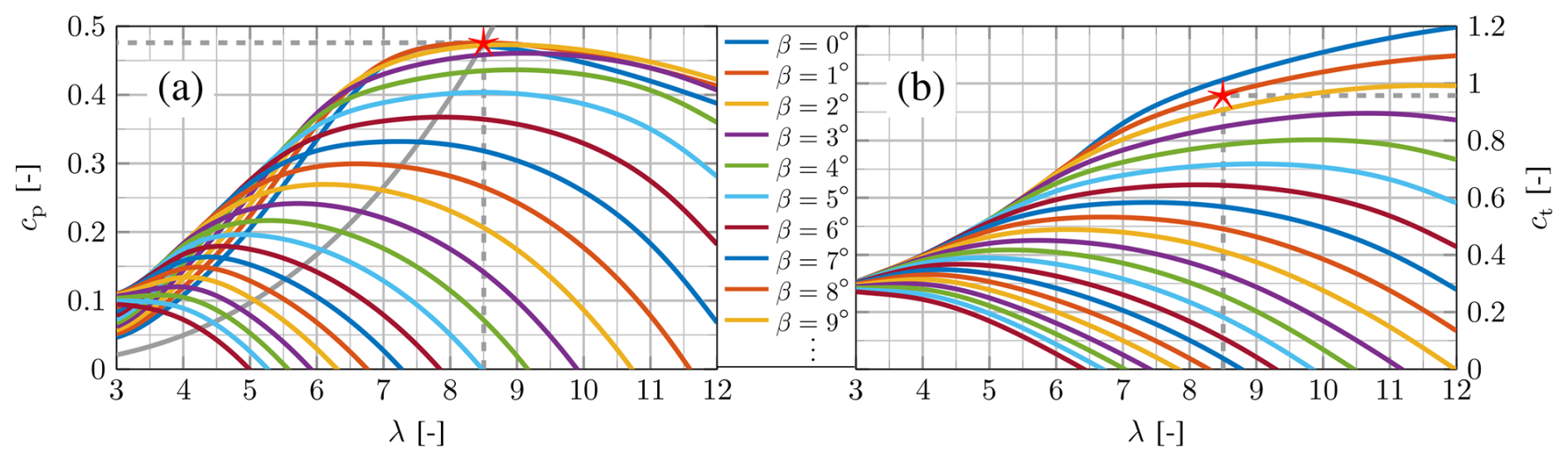
Figure 6 Power coefficient c_p (a) and thrust coefficient c_t (b) as functions of tip speed ratio λ and blade pitch angle β. The MPP is indicated with the symbol . $({\mathit{\lambda }}^{\star },{\mathit{\beta }}^{\star })=(\mathrm{8.5},\mathrm{1.1}\mathrm{°})$, $c_{\mathrm{p}}^{\star }=c_{\mathrm{p}}({\mathit{\lambda }}^{\star }$, ${\mathit{\beta }}^{\star })=\mathrm{0.48}$, $c_{\mathrm{t}}^{\star }=c_{\mathrm{t}}({\mathit{\lambda }}^{\star }$, and ${\mathit{\beta }}^{\star })=\mathrm{0.96}$.

The operating limits are set as follows: ${\mathrm{\Omega }}_{min}=\mathrm{30.81}\mathit{\%}$, $P_{\mathrm{e},max}=\mathrm{105}\mathit{\%}$, $M_{\mathrm{e},max}=\mathrm{106}\mathit{\%}$, and ${\dot{M}}_{\mathrm{e},max}=\mathrm{150}\mathrm{\%}{\mathrm{s}}^{-\mathrm{1}}$. The power limit $P_{\mathrm{e},max}$ is chosen based on the inverter design (Höhn et al., 2024), whereas the other limits are chosen based on the aeroelastic design (Bortolotti et al., 2019).

The pitch controller was modified not to include a tip speed constraint below rated wind speed. Thus, at the rated wind speed $v_{\mathrm{w},\mathrm{R}}=\mathrm{9.8}\mathrm{m}{\mathrm{s}}^{-\mathrm{1}}$, the WT operates at its MPP with optimal tip speed ratio ${\mathit{\lambda }}^{\star }=\mathrm{8.5}$. Consequently, the rated tip speed ${\mathit{\omega }}_{\mathrm{R}}r={\mathit{\lambda }}^{\star }{v}_{\mathrm{w},\mathrm{R}}=\mathrm{83.3}\mathrm{m}{\mathrm{s}}^{-\mathrm{1}}$ (slightly) exceeds the tip speed limit of 80 m s⁻¹ assumed in Bortolotti et al. (2019). The resulting rated WT rotor speed ω_R is ca. 4.2 % larger than the rated value in Bortolotti et al. (2019) but still ca. 5.3 % smaller than the maximum assumed rotor speed limit. The higher-speed rating increases not only the rated power but also the rated kinetic energy reserve for inertia provision compared with Bortolotti et al. (2019). Neglecting for simplicity any conversion losses from mechanical to electrical power, the WT physical inertia constant at rated speed is

$$\begin{array}{}\text{(22)}& H_{\mathrm{R}}={\displaystyle \frac{\frac{\mathrm{1}}{\mathrm{2}}\mathrm{\Theta }{{\mathit{\omega }}_{\mathrm{R}}}^{\mathrm{2}}}{p_{\mathrm{R}}}}=\mathrm{3.26}\mathrm{s}.\end{array}$$

The WTs are arranged in an irregular WF layout on semi-complex terrain characterized by gently rolling hills. Figure 7 shows the WF layout and the resulting wake interactions among the WTs in exemplary wind conditions.

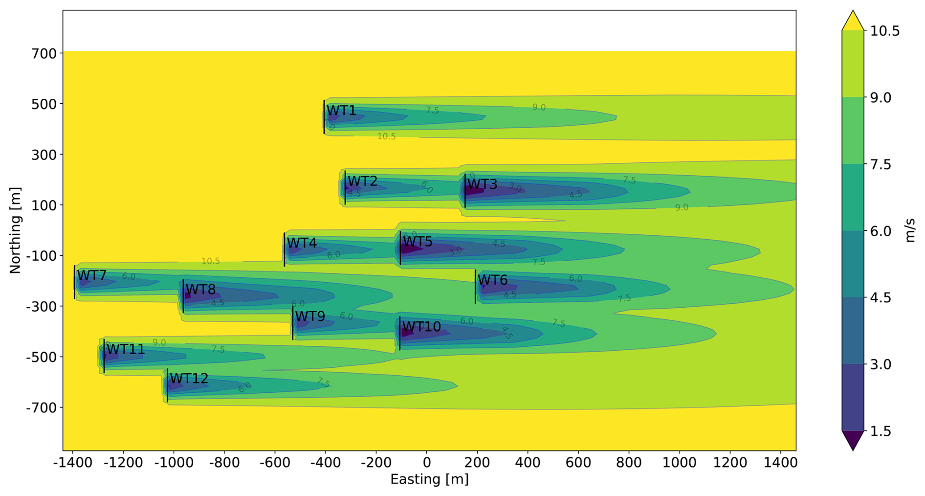
Figure 7 Wind farm layout and wake interactions for ambient wind speed $v_{\mathrm{w}}=\mathrm{11}\mathrm{m}{\mathrm{s}}^{-\mathrm{1}}$ and wind direction Γ_w=270°.

Historical data consisting of 2 years of site-specific weather condition measurements are used to train the data-driven weather forecast model. A deterministic model and a probabilistic model predict the weather conditions with a 15 min resolution for the hour ahead. The deterministic model outputs the expected wind conditions for WF inertia forecasting, whereas the probabilistic model additionally considers the wind condition uncertainties, enabling uncertainty quantification of the predicted WF inertia.

4.1 WT steady states

The WT steady states depend on the WT operating point (v_w,P_set), defined by wind speed v_w and power setpoint P_set. Although the WT steady states generally depend on the pairs (v_w,P_set), they are calculated by solving one-dimensional optimization (sub)problems. This is obtained through a case analysis of active operating constraints, which is described in Appendix I. This enables the fast initialization of the WT dynamic model without running time-consuming simulations until reaching steady state. Figure 8 illustrates the WT steady-state conditions as a function of v_w, with P_set ranging from the minimum considered value of 90 % (dark blue line) in increments of 1 % up to the maximum value of 100 % (dark red line). Note that P_set=1 corresponds to MPPT, and P_set<1 corresponds to MRS-based derating. In Fig. 8 (and in all following figures), all normalized quantities (indicated by %) are in per unit of rated values; e.g., $F_{\mathrm{t},\text{pu}}:=F_{\mathrm{t}}/F_{\mathrm{t},\mathrm{R}}$ with thrust force $F_{\mathrm{t}}=F_{\mathrm{t},\mathrm{R}}$ at the rated WT operating point $(v_{\mathrm{w}}=v_{\mathrm{w},\mathrm{R}}=\mathrm{9.8}\mathrm{m}{\mathrm{s}}^{-\mathrm{1}},P_{\text{set}}=\mathrm{1})$. The only exception is the power setpoint P_set defined in per unit of available power ${\stackrel{\mathrm{‾}}{P}}^{\star }$; see Eq. (9).

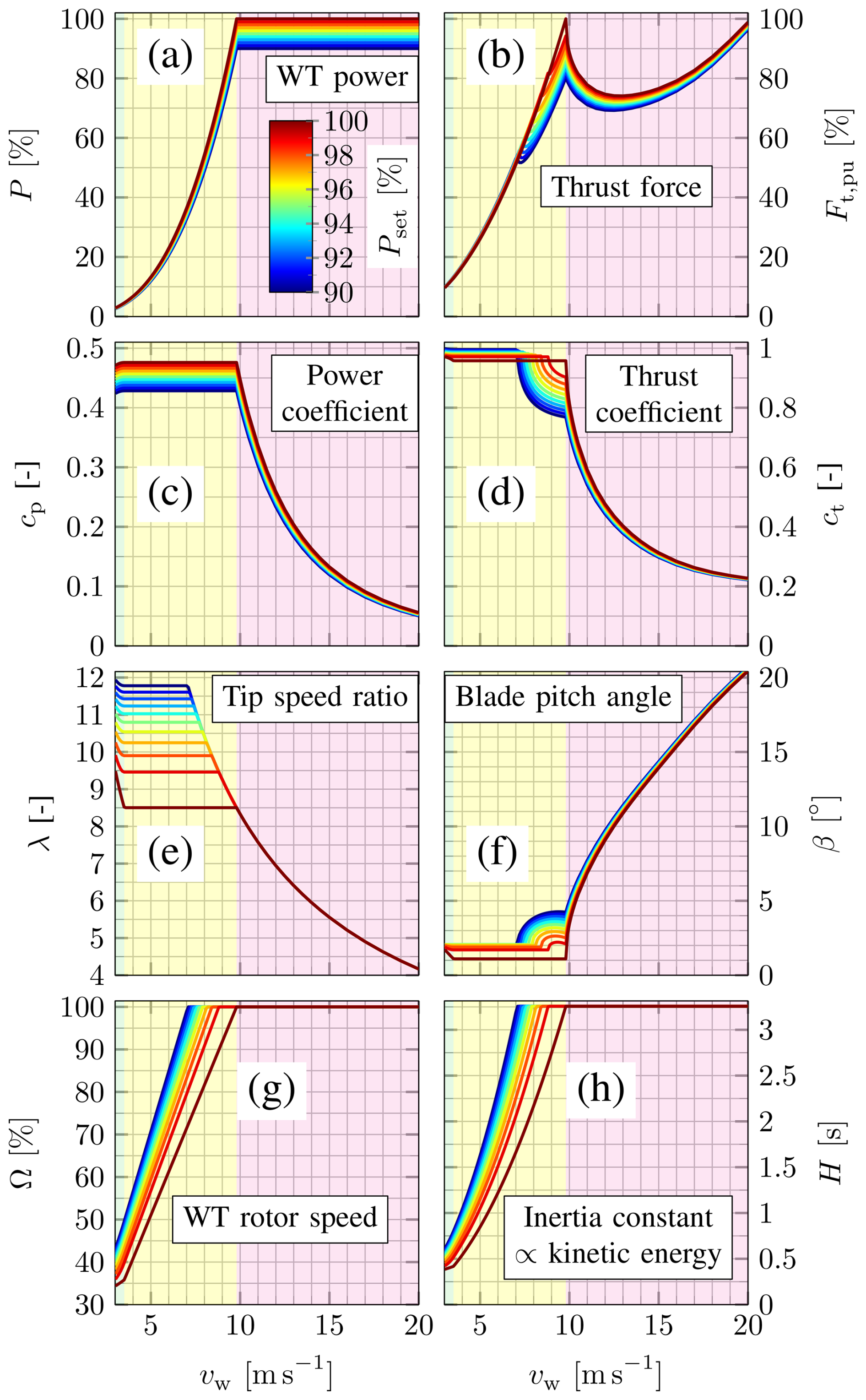
Figure 8 WT steady-state conditions as functions of wind speed v_w for MRS-based derating with power setpoint P_set (see steady-state calculation in Appendix I).

In Fig. 8, a higher derating or a lower P_set increases the WT rotor speed Ω at low wind speeds, e.g., at $v_{\mathrm{w}}=\mathrm{5}\mathrm{m}{\mathrm{s}}^{-\mathrm{1}}$, such that the kinetic energy or physical inertia constant H increases proportionally to Ω². For P_set=1 (MPPT), the blade pitch angle equals its optimal value for below-rated wind speeds in region II; i.e., $\mathit{\beta }={\mathit{\beta }}^{\star }=\mathrm{1.1}\mathrm{°}$ (see also Fig. 6). On the other hand, for above-rated wind speeds in region III, β increases to limit the WT rotor speed to Ω=1. In addition to Ω, the pitch control requires v_w as input (see Fig. 2) to adjust the lower pitch angle limit as a function of the tip speed ratio $\mathit{\lambda }=\mathrm{\Omega }{\mathit{\omega }}_{\mathrm{R}}r/v_{\mathrm{w}}$; i.e., ${\mathit{\beta }}_{\text{ref}}\ge {\mathit{\beta }}_{min}\left(\mathit{\lambda }\right):=\text{arg\hspace{0.17em}max}{c}_{\mathrm{p}}(\mathit{\lambda },\mathit{\beta })$. Considering the plots in the third row of Fig. 8, this β_min adjustment is only relevant for $\mathit{\lambda }>{\mathit{\lambda }}^{\star }=\mathrm{8.5}$ due to constant ${\mathit{\beta }}_{min}={\mathit{\beta }}^{\star }$ elsewhere. More precisely, for P_set=1 (MPPT), the β_min adjustment is only relevant in the small transition region I–II near $v_{\mathrm{w},\text{cut-in}}=\mathrm{3.02}\mathrm{m}{\mathrm{s}}^{-\mathrm{1}}$; however, for P_set<1 (derating), the β_min adjustment is also relevant in region II, as the increased tip speed ratio $\mathit{\lambda }>{\mathit{\lambda }}^{\star }$ leads to a higher blade pitch angle $\mathit{\beta }={\mathit{\beta }}_{min}\left(\mathit{\lambda }\right)\ge {\mathit{\beta }}^{\star }$.

In Fig. 8, after reaching rated rotor speed Ω=1, the tip speed ratio decreases with increasing wind speed, i.e., $\mathit{\lambda }\propto {v_{\mathrm{w}}}^{-\mathrm{1}}$, and the blade pitch angle β increases to limit the rotor speed to Ω=1. Both decreasing λ and increasing β reduce the thrust coefficient c_t (at least near the optimal operating point; see also Fig. 6). Note that, for MRS-based derating (P_set<1), the rotor speed reaches Ω=1 at below-rated wind speeds $v_{\mathrm{w}}<v_{\mathrm{w},\mathrm{R}}$. For Ω<1 and constant P_set, the thrust coefficient c_t is constant due to constant λ and β. For Ω<1 and varying P_set, e.g., at $v_{\mathrm{w}}=\mathrm{5}\mathrm{m}{\mathrm{s}}^{-\mathrm{1}}$, higher derating increases λ but only slightly increases $\mathit{\beta }={\mathit{\beta }}_{min}\left(\mathit{\lambda }\right)$ such that c_t (slightly) increases. This (slightly) increases the thrust force F_t,pu, although the changes are negligible. In contrast, for initial operation with maximum speed Ω=1 at higher or above-rated wind speeds, higher derating significantly reduces the thrust force due to increasing β but constant λ.

To summarize, the MRS-based derating significantly decreases the thrust force for Ω=1, i.e., if no further rotor acceleration is feasible. This is in line with the observed reduction in damage equivalent loads during derating, as reported by Aho et al. (2014). Otherwise, for Ω<1, i.e., especially at low wind speeds or for minor derating in region II, the MRS-based derating accelerates the rotor, but the resulting increase in thrust force is negligible.

4.2 WT inertia provision for the reference frequency event

This section evaluates WT grid-forming capabilities in terms of maximum inertia provision as a function of WT operating point (v_w,P_set). At first, Sect. 4.2.1 introduces the considered reference frequency event defined by the German grid code and derives a worst-case test scenario for WT inertia provision. Then, Sect. 4.2.2 discusses the resulting dynamic WT simulations for optimized inertia provision, i.e., for $H_{\mathrm{v}}=H_{\mathrm{v},max}$, with and without MRS-based derating. Finally, Sect. 4.2.3 discusses the mapping of WT operating points to the maximum feasible inertia constant over a wide operating range.

4.2.1 Grid codes

Although grid codes can vary among countries and system operators, the core requirements for inertia provision are similar (Ghimire et al., 2025). This paper focuses on the German code for grid-forming control and its requirements for inertia provision (VDE, 2024a, b). This grid code defines two reference frequency events with maximum initial ROCOF magnitudes of $\left|{\dot{f}}_{\mathrm{s}}\right|=\mathrm{2}\mathrm{Hz}{\mathrm{s}}^{-\mathrm{1}}$: one for negative inertia provision due to a high positive initial ROCOF and another for positive inertia provision due to a high negative initial ROCOF. The latter is considered the worst-case reference frequency event for WFs, since the output power has to increase for inertia provision, which decelerates the WTs. Emulating this reference frequency event and evaluating the WF power response are required to verify inertia provision.

The considered grid code (VDE, 2024b) defines various tests based on the reference frequency events to verify inertia provision, including operation in (i) fictive or simulated island mode with changing power imbalance ΔP due to varying electrical load; (ii) grid-emulator-connected mode with changing ROCOF ${\dot{\mathrm{\Omega }}}_{\mathrm{s}}$; and (iii) real grid-connected mode with changing controller-internal ROCOF, corresponding to the VSM acceleration ${\dot{\mathrm{\Omega }}}_{\mathrm{v}}$ (see also Fig. 4). In the latter case (iii), the frequency signal defined by the reference frequency events is added as a disturbance to the controller-internal frequency, corresponding to the VSM speed Ω_v. It should be noted that some tests consider deactivated droop control. However, the verification principle is always the same; see also Schöll et al. (2024). In all tests, a ROCOF changes $\dot{\mathrm{\Omega }}$, and the inertial power response ΔP is measured or vice versa. The actual inertia provision is quantified by the measured inertia constant $H_{\text{meas}}=|\mathrm{\Delta }P/(\mathrm{2}\dot{\mathrm{\Omega }}\left)\right|$ at quasi-steady state, as obtained from Eq. (1a). Note that ΔP corresponds to the measured power change ΔP_meas only if droop control is deactivated. Otherwise, for the correct calculation of H_meas, the droop power change $\mathrm{\Delta }{\stackrel{\mathrm{‾}}{P}}_{\mathrm{d}}$ (depending on the frequency deviation) should be added to the inertial power (depending on the ROCOF) during the frequency event; i.e., $\mathrm{\Delta }P=\mathrm{\Delta }{P}_{\text{meas}}-\mathrm{\Delta }{\stackrel{\mathrm{‾}}{P}}_{\mathrm{d}}$. Clearly, H_meas must match the expected VSM inertia constant; i.e., H_meas≈H_v.

For the considered VSM control, H_meas≈H_v holds if no power saturation is active (see also Fig. 5). In other words, it is assumed that the actual VSM control implementation would pass all tests (VDE, 2024b) with H_meas≈H_v for an arbitrarily chosen H_v if no power saturation exists. It follows that H_meas≈H_v holds if no operating limits are violated in the simulations of the WT model. Otherwise, in reality, the protection methods would saturate the output power as the desired inertia provision is not feasible; i.e., H_meas<H_v due to $H_{\mathrm{v}}>H_{\mathrm{v},max}$. Thus, assuming proper VSM control allows this study to focus on the relevance of interactions with WT control, WT characteristics, and operating limits.

Running and passing all tests defined in the grid code (VDE, 2024b) verifies proper grid-forming control implementation and inertia provision for a given H_v at a given operating point. However, this approach is not suitable for evaluating the maximum feasible inertia provision of WFs over a wide operating range. Thus, this paper considers a single worst-case test scenario to simulate WTs for varying H_v and varying operating point (v_w,P_set). The reference frequency event for positive inertia provision with an initial ROCOF of ${\dot{f}}_{\mathrm{s}}=-\mathrm{2}\mathrm{Hz}{\mathrm{s}}^{-\mathrm{1}}$ (VDE, 2024b) defines the input ${\dot{\mathrm{\Omega }}}_{\mathrm{s}}$ in Fig. 2. This can be interpreted as ideal ROCOF emulation at the point of common coupling. As in real grid-connected operation mode, droop control is activated. Finally, a WT survives the worst-case test scenario if no operating limit is violated, i.e., for $H_{\mathrm{v}}\le H_{\mathrm{v},max}$ at a given operating point (v_w,P_set), according to Eq. (14).

4.2.2 Optimized time response

This section considers simulation results of the WT inertial response to the reference frequency event with optimized $H_{\mathrm{v}}=H_{\mathrm{v},max}$ at $v_{\mathrm{w}}=\mathrm{9}\mathrm{m}{\mathrm{s}}^{-\mathrm{1}}<v_{\mathrm{w},\mathrm{R}}$ for two different power setpoints: (i) P_set=100 % for MPPT in Fig. 9 and (ii) P_set=95 % for MRS-based derating in Fig. 10. The grid frequency is identical in both cases (panel a); i.e., Ω_s decreases with the initial ROCOF ${\dot{\mathrm{\Omega }}}_{\mathrm{s}}=-\mathrm{4}\mathrm{\%}{\mathrm{s}}^{-\mathrm{1}}$ for $t_{\mathrm{0}}=\mathrm{0}\mathrm{s}\le t<\mathrm{1}\mathrm{s}$ and further decreases with ${\dot{\mathrm{\Omega }}}_{\mathrm{s}}=-\mathrm{2}/\mathrm{3}\mathrm{\%}{\mathrm{s}}^{-\mathrm{1}}$ afterwards, until reaching the nadir ${\mathrm{\Omega }}_{\mathrm{s},min}=\mathrm{95}\mathit{\%}$ at $t_{\mathrm{s},min}=\mathrm{2.5}\mathrm{s}$. Then, Ω_s increases with ${\dot{\mathrm{\Omega }}}_{\mathrm{s}}=\mathrm{2}\mathrm{\%}{\mathrm{s}}^{-\mathrm{1}}$, before staying constant at Ω_s=98 % for t≥4 s. In addition, panel (a) shows the VSM speed Ω_v, the WT speed Ω, and the adjusted MPPT input Ω_H0. Panel (b) shows the mechanical power P_m, the electrical power P_e, the electrical torque M_e, and its limit $M_{\mathrm{e},max}$. Panels (d), (e), and (f) show the tip speed ratio λ, the power coefficient c_p, and the blade pitch angle β, respectively. Finally, panel (c) shows the resulting aerodynamic trajectory (red line).

Figure 9 WT simulation results for MPPT at $(v_{\mathrm{w}}=\mathrm{9}\mathrm{m}{\mathrm{s}}^{-\mathrm{1}},P_{\text{set}}=\mathrm{100}\mathit{\%})$ with optimized $H_{\mathrm{v},max}=\mathrm{2.26}\mathrm{s}$.

Figure 10 WT simulation results for MRS-based derating at $(v_{\mathrm{w}}=\mathrm{9}\mathrm{m}{\mathrm{s}}^{-\mathrm{1}},P_{\text{set}}=\mathrm{95}\mathit{\%})$ with optimized $H_{\mathrm{v},max}=\mathrm{3.80}\mathrm{s}$.

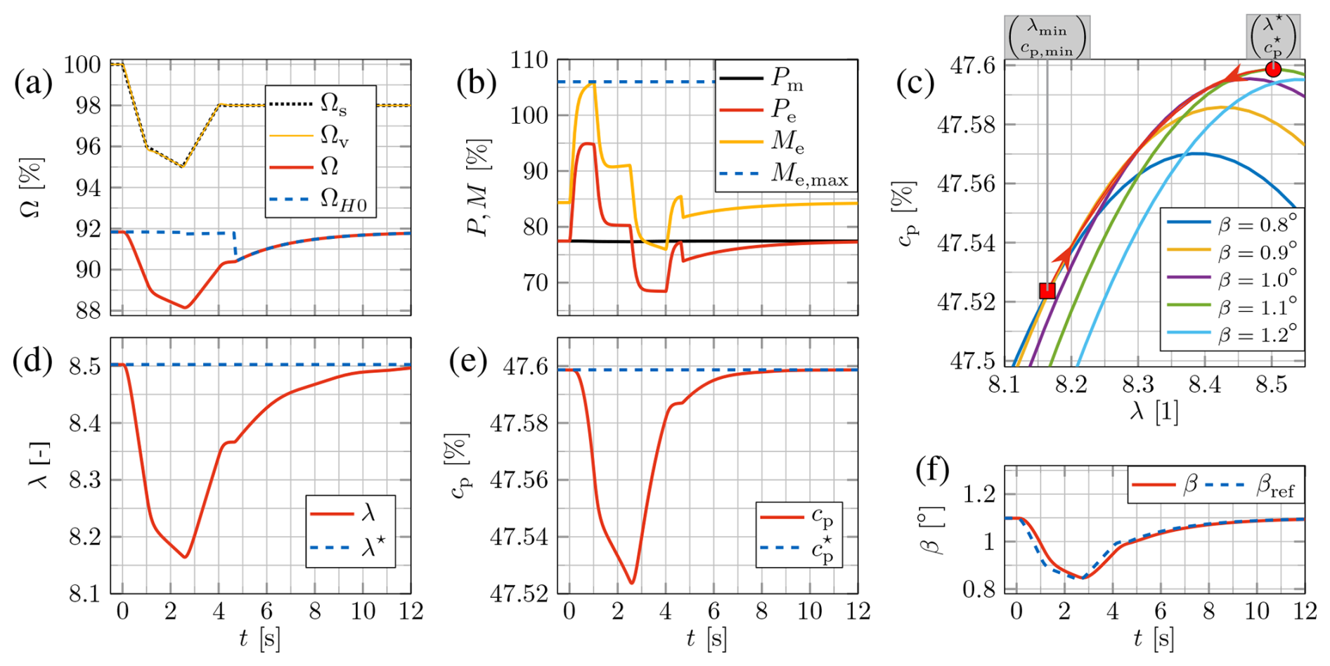
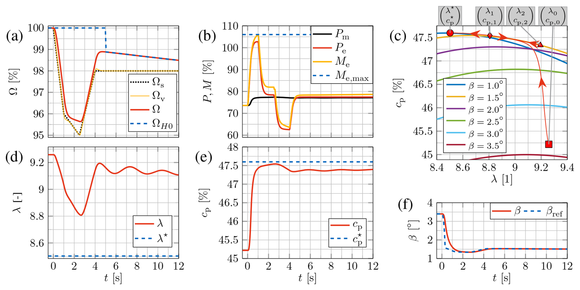
In Fig. 9, the power coefficient starts at its maximum value due to MPPT, i.e., $(\mathit{\beta },\mathit{\lambda })=({\mathit{\beta }}^{\star },{\mathit{\lambda }}^{\star })$, which yields $c_{\mathrm{p}}=c_{\mathrm{p}}^{\star }$. The VSM inertial response increases the electrical power P_e during the negative ROCOF, whereas the aerodynamic or mechanical power P_m remains almost constant. Thus, the WT rotor decelerates, and the tip speed ratio λ decreases. After the ROCOF changes from negative to positive at $t_{\mathrm{s},min}=\mathrm{2.5}\mathrm{s}$, P_e rapidly decreases below P_m, and the rotor accelerates. Accordingly, considering the trajectory (c_p,λ) in Fig. 9c, the WT leaves its MPP $({\mathit{\lambda }}^{\star },c_{\mathrm{p}}^{\star })$ during the negative ROCOF, with significantly decreasing λ but almost constant c_p. Due to the grid synchronization delay of the VSM, the WT reaches its rotor speed nadir or $({\mathit{\lambda }}_{min},c_{\mathrm{p},min})$ at t=2.593 s, i.e., shortly after the frequency nadir at $t_{\mathrm{s},min}=\mathrm{2.5}\mathrm{s}$. Afterwards, with increasing Ω, the trajectory converges to $({\mathit{\lambda }}^{\star },c_{\mathrm{p}}^{\star })$ for t→∞.

At t≈4.65 s in Fig. 9a, the MPPT compensation resets Ω_H0 to Ω such that P_e in panel (b) rapidly decreases to re-accelerate the WT to its MPP, called WT rotor speed recovery. Clearly, decreasing the rate limit ${\dot{\mathrm{\Omega }}}_{H\mathrm{0},max}$ for the transition between active and inactive MPPT compensation in Eq. (13) leads to a smoother change in P_e, which is expected to cause less severe secondary frequency disturbances (Godin et al., 2019). However, this would slow down the WT rotor speed recovery. Finding a reasonable compromise is beyond the scope of this paper, but see Appendix G for further discussion on this point.

In Fig. 10, the initial steady-state power P_m(t₀)=P_e(t₀) is 5 % below its initial MPP value in Fig. 9 due to P_set=95 % or $c_{\mathrm{p}}\left(t_{\mathrm{0}}\right)=\mathrm{95}\mathit{\%}\cdot c_{\mathrm{p}}^{\star }$ for t₀=0. Note that the lower initial electromagnetic torque M_e(t₀) leads to (i) higher initial WT speed Ω(t₀)=1 in Fig. 10 compared with Ω(t₀)=91.8 % in Fig. 9 and (ii) active pitch control; i.e., $\mathit{\beta }\left(t_{\mathrm{0}}\right)>{\mathit{\beta }}^{\star }$ in Fig. 10. The trajectory (c_p,λ) in Fig. 10c starts at $({\mathit{\lambda }}_{\mathrm{0}},c_{\mathrm{p},\mathrm{0}})$ with ${\mathit{\lambda }}_{\mathrm{0}}>{\mathit{\lambda }}^{\star }$ and $c_{\mathrm{p},\mathrm{0}}<c_{\mathrm{p}}^{\star }$. The VSM inertial response increases the electromagnetic power P_e during the negative ROCOF so that the WT decelerates and λ decreases. At the same time, the pitch control decreases β due to Ω<1. The trajectory reaches the (local) WT rotor speed nadir or $({\mathit{\lambda }}_{\mathrm{1}},c_{\mathrm{p},\mathrm{1}})$ at t≈2.62 s. Afterwards, during the positive ROCOF, P_e rapidly decreases such that λ increases, reaching $({\mathit{\lambda }}_{\mathrm{2}},c_{\mathrm{p},\mathrm{2}})$ at t≈4.44 s. Finally, during constant but below-rated frequency Ω_s<1 for t≥4, inertia provision is inactive, but the active power droop control increases P_e to the maximum available MPPT power, which is greater than the initial value P_e(t₀). Thus, (c_p,λ) converges to the MPP $({\mathit{\lambda }}^{\star },c_{\mathrm{p}}^{\star })$ for t→∞. Note that the trajectory in Fig. 10 converges to the MPP from the right side of the MPP, whereas, for P_set=100 % in Fig. 9, the trajectory converges to the MPP from the left side of the MPP.

After the ROCOF changes from negative to positive at t=2.5 s in Fig. 10d, the electrical power $P_{\mathrm{e}}\approx P_{\text{ref}}={\stackrel{\mathrm{‾}}{P}}_{\text{set}}^{\star }+P_{\mathrm{v}}+{\stackrel{\mathrm{‾}}{P}}_{\mathrm{d}}$ (panel b) decreases as the VSM inertial power becomes negative; i.e., P_v<0. At the same time, the droop power increases as power reserves become available; i.e., ${\stackrel{\mathrm{‾}}{P}}_{\mathrm{d}}=P_{\mathrm{d},max}>\mathrm{0}$. The droop power ${\stackrel{\mathrm{‾}}{P}}_{\mathrm{d}}>\mathrm{0}$ counteracts the VSM inertial power P_v<0 during the grid frequency recovery. Thus, both droop control and inertia provision are active at the minimum P_e at t=4 s in Fig. 10b, whereas ${\stackrel{\mathrm{‾}}{P}}_{\mathrm{d}}=P_{\mathrm{d},max}=\mathrm{0}$ and P_v>0 holds for the maximum P_e at t=1 s.

Considering Figs. 9 and 10 (panel b), the electromagnetic torque M_e reaches its limit $M_{\mathrm{e},max}$ in both cases; i.e., the second constraint of the optimization problem Eq. (14) is active. However, the initial torque M_e(t₀) for 5 % power derating in Fig. 10b is more than 12 % lower than M_e(t₀) for MPPT in Fig. 9b. The torque reduction is higher than the power derating due to an 11 % higher initial rotor speed Ω(t₀) in Fig. 10a than in Fig. 9a. Clearly, the MRS-based derating maximizes the torque headroom $M_{\mathrm{e},max}-M_{\mathrm{e}}\left(t_{\mathrm{0}}\right)$ for inertia provision by maximizing the rotor speed.

In general, the VSM inertial response to the initial negative ROCOF increases the electrical power P_e, which decelerates the rotor in both cases (Figs. 9 and 10). However, due to a higher initial value, the rotor speed does not fall below its MPP value Ω=91.84 % for MRS-based derating in Fig. 10; on the other hand, Ω decreases to 88.15 % for MPPT in Fig. 9. Moreover, the WT rotor deceleration leads to constant (or only slightly decreasing) mechanical power P_m in Fig. 9 but increasing P_m in Fig. 10. Consequently, the MRS-based derating strategy provides both additional kinetic energy and additional wind energy reserves for inertia provision.

To summarize, the optimized values for the VSM inertia constant $H_{\mathrm{v}}=H_{\mathrm{v},max}$ are 2.26 and 3.80 s for P_set=100 % (MPPT) in Fig. 9 and for P_set=95 % (MRS-based derating) in Fig. 10, respectively. For these two exemplary operating points, the MRS-based derating of 5 % increases the inertia provision capability in terms of $H_{\mathrm{v},max}$ by ca. $\mathrm{3.80}/\mathrm{2.26}-\mathrm{1}\approx \mathrm{68}\mathit{\%}$ compared with MPPT.

4.2.3 Mapping of WT operating points

The proposed WF inertia forecasting approach uses LUTs to map the operating points of all WTs to the WF inertia, assuming optimal tuning $H_{\mathrm{v}}=H_{\mathrm{v},max}$ for each WT in the WF. For the proposed solution of the optimization problem in Eq. (14), Fig. 11 depicts the resulting LUTs of the form $H_{\mathrm{v},max}=f(v_{\mathrm{w}},P_{\text{set}})$ for all operating points (v_w,P_set) within the range $v_{\mathrm{w},\text{cut-in}}\le v_{\mathrm{w}}\le \mathrm{15}\mathrm{m}{\mathrm{s}}^{-\mathrm{1}}$ and $\mathrm{90}\mathit{\%}\le P_{\text{set}}\le \mathrm{100}\mathit{\%}$. For enhanced visualization and clarity, panels (a) and (b) show the same results from different points of view. In the 2-D plot (panel a), the color coding for the power setpoint P_set is the same as in Fig. 8; in the 3-D plot (panel b), the datapoint colors indicate the active optimization constraints in Eq. (14).

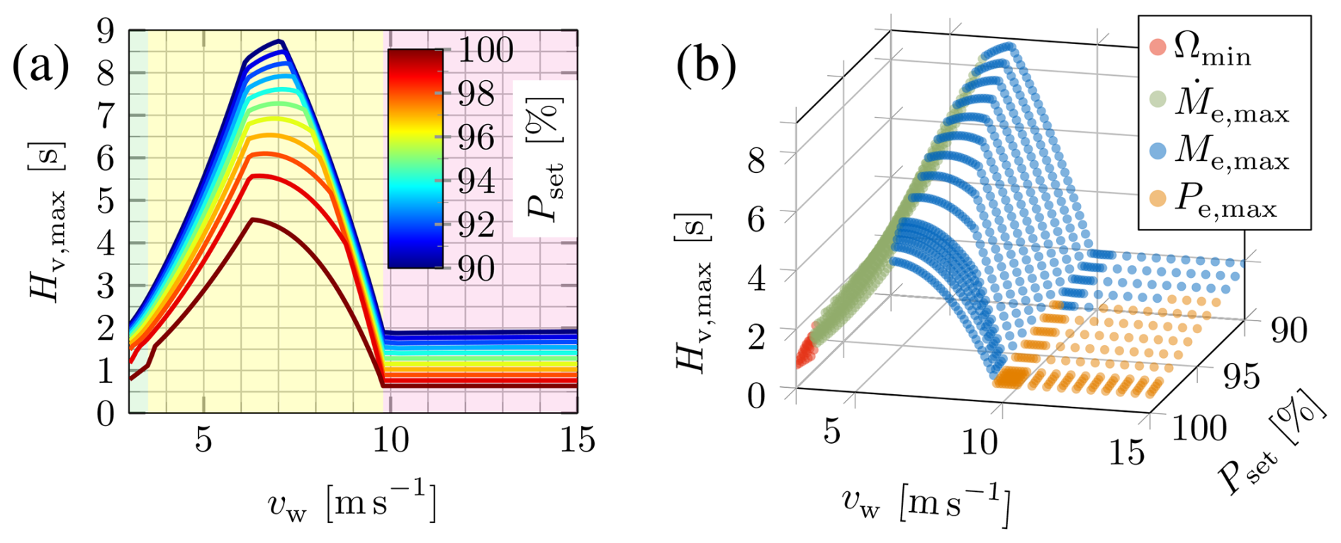
Figure 11 Maximum inertia provision at different operating points (v_w,P_set), with active constraints highlighted in panel (b).

The LUTs were computed on a standard desktop computer (FUJITSU Workstation CELSIUS W580, Xeon E-2246G 6C 3.60 GHz 12 MB, 2 × 16 GB DDR4-2666, NVIDIA Quadro P1000 4 GB) using MATLAB's Parallel Computing Toolbox, Optimization Toolbox, and Simulink. Four CPU cores were used in parallel via a “parfor” loop (MATLAB, 2025c) to perform solver-based nonlinear optimizations (MATLAB, 2025b), including numerous WT simulations executed in Simulink's rapid accelerator mode (MATLAB, 2025a). The computation time depended strongly on the simulation and solver settings, in particular the optimality and constraint tolerances. Without any attempt at optimizing the software for numerical efficiency, the wall-clock time was typically of the order of 4 h for a complete LUT generation. Although execution time is a metric that quickly becomes obsolete and is influenced by many factors, the computational cost of the proposed method is acceptable for realistic applications, especially since the LUT generation is performed offline rather than during operation.

In Fig. 11, the rotor speed limit Ω_min is only active for low wind speeds near v_w,cut-in. For most operating points characterized by $v_{\mathrm{w}}<\mathrm{6.3}\mathrm{m}{\mathrm{s}}^{-\mathrm{1}}$, the torque rate limit ${\dot{M}}_{\mathrm{e},max}$ constraint is active. For P_set=1, i.e., even without derating, the maximum inertia constant $H_{\mathrm{v},max}=\mathrm{4.55}\mathrm{s}$ at $v_{\mathrm{w}}=\mathrm{6.3}\mathrm{m}{\mathrm{s}}^{-\mathrm{1}}$ exceeds the rated WT physical inertia constant H_R=3.26 s. However, for $\mathrm{6.3}\mathrm{m}{\mathrm{s}}^{-\mathrm{1}}<v_{\mathrm{w}}\le v_{\mathrm{w},\mathrm{R}}$, the torque limit $M_{\mathrm{e},max}$ reduces $H_{\mathrm{v},max}$ with increasing wind speed. For above-rated wind speeds $v_{\mathrm{w}}>v_{\mathrm{w},\mathrm{R}}$ and P_set=1, the virtual inertia constant $H_{\mathrm{v},max}$ is smaller than the WT physical inertia constant H=H_R due to the electrical power limit $P_{\mathrm{e},max}$. The MRS-based derating increases $H_{\mathrm{v},max}$ over the complete wind speed range.

Appendix J reports the $H_{\mathrm{v},max}$ results obtained with the simplified solution derived in Sect. 3.4.2 and compares them with the complete numerical solution. Appendix G reports the results obtained with an additional (optional) constraint for WT rotor speed recovery.

For each operating point (v_w,P_set) and corresponding optimal $H_{\mathrm{v}}=H_{\mathrm{v},max}$ tuning, the rotor speed nadir minΩ and the mechanical power extrema minP_m or maxP_m are evaluated in the inertial response time interval defined in Appendix Eq. (K1). Figure 12a shows the normalized deviation of minΩ to the initial WT speed Ω₀ (i.e., $(min\mathrm{\Omega }-{\mathrm{\Omega }}_{\mathrm{0}})/{\mathrm{\Omega }}_{\mathrm{0}}$) and Fig. 12b shows the normalized deviation of minΩ to the MPP speed Ω_mpp (i.e., $(min\mathrm{\Omega }-{\mathrm{\Omega }}_{\text{mpp}})/{\mathrm{\Omega }}_{\text{mpp}}$, where Ω_mpp:=Ω₀ for P_set=1). Figure 13a and b show the normalized deviation of minP_m and maxP_m to the initial WT mechanical power P_m,0, i.e., $(min{P}_{\mathrm{m}}-P_{\mathrm{m},\mathrm{0}})/P_{\mathrm{m},\mathrm{0}}$ and $(max{P}_{\mathrm{m}}-P_{\mathrm{m},\mathrm{0}})/P_{\mathrm{m},\mathrm{0}}$, respectively.

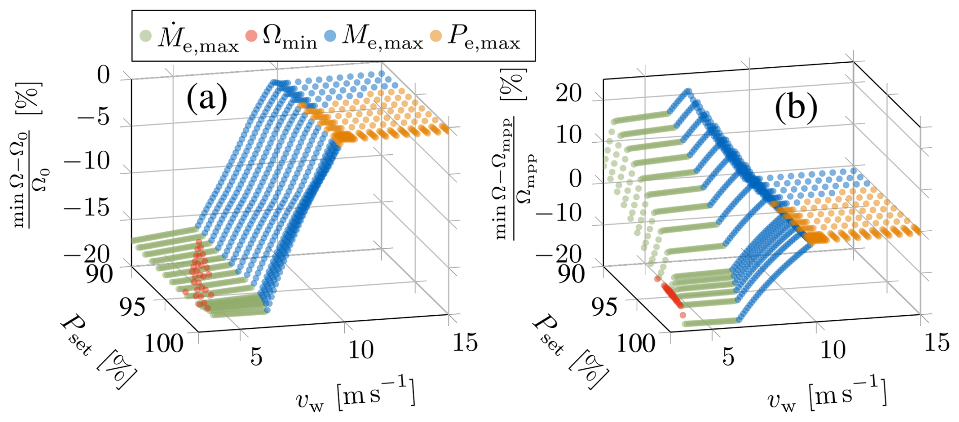
Figure 12 WT rotor speed nadir: deviation from the initial operating point (a) and the MPP (b).

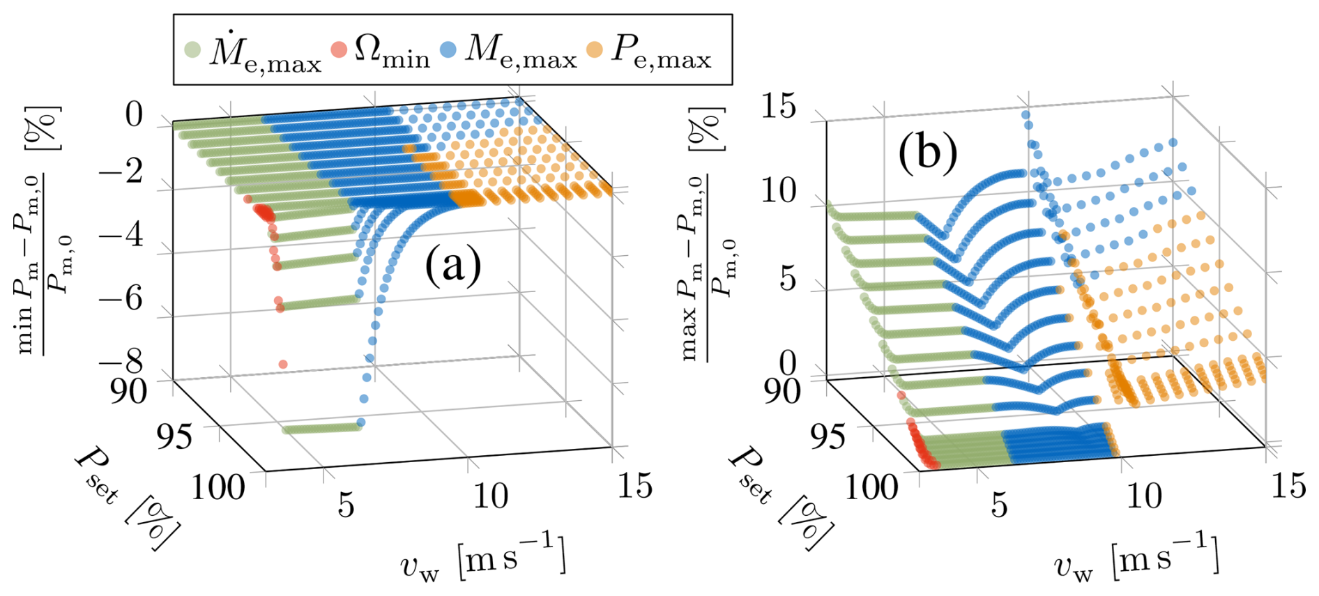
Figure 13 WT mechanical power extrema: minimum (a) and maximum (b) deviation from the initial operating point.

The WT significantly decelerates during the inertial response at low wind speeds, although the rotor speed deviation does not exceed 20 % of Ω₀ in Fig. 12a. Clearly, the lower speed limit Ω_min is only relevant for a few operating points at low wind speeds and minor derating; i.e., for all other operating points the available kinetic energy reserve cannot be fully extracted for inertia provision due to active torque or power constraints. Decreasing P_set increases Ω₀ such that the rotor speed does not fall below its MPP value if the derating is high enough, i.e., for $min\mathrm{\Omega }-{\mathrm{\Omega }}_{\text{mpp}}>\mathrm{0}$ in Fig. 12b. In this case, no rotor speed recovery is needed after the inertial response.

For MPPT, the rotor deceleration decreases the power coefficient c_p. Thus, the aerodynamic power decreases during the inertial response; i.e., $min{P}_{\mathrm{m}}<P_{\mathrm{m},\mathrm{0}}$ for P_set=1 at below-rated wind speeds in Fig. 13a. However, minor derating significantly increases minP_m. For P_set≤95 %, the reduction in P_m is negligible due to $min\mathrm{\Omega }\approx {\mathrm{\Omega }}_{\text{mpp}}$, or P_m even increases due to $min\mathrm{\Omega }>{\mathrm{\Omega }}_{\text{mpp}}$, as shown in Figs. 12b and 13a. In summary, the MRS-based derating leads to less severe rotor deceleration due to higher initial rotor speed and thus also higher aerodynamic power during the inertial response.

4.3 WF inertia monitoring and forecasting

Applying the proposed approach to a real WF ambient wind profile over 5 d, the figures that follow illustrate the following:

1. actual and forecasted WF ambient wind condition inputs for the wake model (Fig. 14);

2. WF inertia monitoring results, i.e., WF inertia calculations based on actual wind conditions (Figs. 15 and 16);

3. WF inertia forecasting results, i.e., WF inertia calculations based on predicted wind conditions (Fig. 17);

4. uncertainties due to WF ambient wind forecast errors, wake model errors, and WT inertia provision errors (Figs. 17–19).

In addition to the actual WF ambient wind speed and direction, Fig. 14a shows the different hour-ahead forecasts. The wind speed v_w values of the deterministic (“Det”) forecast lie between the values of the probabilistic minimal (“Pro Min”) forecast and the probabilistic maximal (“Pro Max”) forecast. The forecast for the wind direction Γ_w in Fig. 14b is deterministic. All forecast trends match the actual data. The following WF simulation results are based on actual and forecasted WF ambient wind data for inertia monitoring and forecasting, respectively.

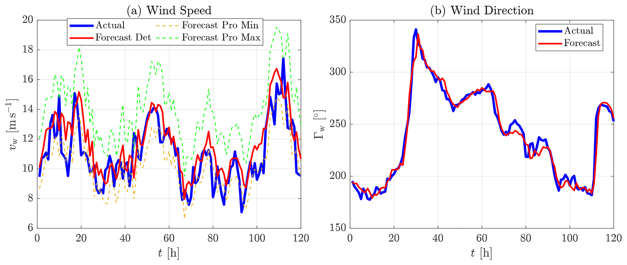
Figure 14 Ambient wind conditions and its hour-ahead forecasts: wind speed (a) and wind direction (b) for actual measurements (Actual) as well as for deterministic (“Det”), probabilistic minimal (“Pro Min”), and probabilistic maximal (“Pro Max”) forecasts.

In Fig. 15a, the maximum (local) wind speed (upper envelope curve) of all 12 WTs (WT1–WT12) equals the actual WF ambient wind speed in Fig. 14. Clearly, wake effects reduce the wind speed for downstream WTs, resulting in a lower mean wind speed in Fig. 15. In Fig. 15b, the normalized WT power at steady state is defined as $P:=P_{\mathrm{e}}=P_{\mathrm{m}}$. Due to the equal power rating of all WTs, the normalized WF power corresponds to the mean normalized WT power, and the WF (virtual) inertia constant corresponds to the mean WT (virtual) inertia constant. For P_set=1, the WF operates at rated WF power P=1 if the local wind speed at all WTs reaches $v_{\mathrm{w}}\ge v_{\mathrm{w},\mathrm{R}}$, e.g., at t=110 h in Fig. 15b. Accordingly, at t=110 h in Fig. 15c, all WTs operate at Ω=1 such that the physical inertia constant H is saturated by its rated value H_R. In contrast, the maximum virtual inertia constant $H_{\mathrm{v},max}$ in Fig. 15d is saturated by its lower limit given by the maximum power constraint (reported earlier in Fig. 11). For lower wind speeds with all WTs operating in region II, e.g., at t=70 h in Fig. 15, the lower WT rotor speeds lead to lower H but higher $H_{\mathrm{v},max}$, as the power constraint becomes inactive. Note that $H_{\mathrm{v},max}>H$ is possible because the WTs rotate asynchronously, whereas the VSMs synchronize with the grid frequency. Thus, for a given ROCOF, a VSM-controlled WT with physical inertia constant H and virtual inertia constant H_v>H may extract more kinetic energy than a (directly grid-connected) SM with the same H.

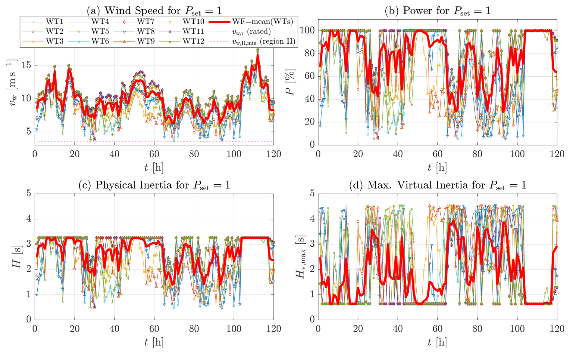
Figure 15 Simulation results for all 12 WTs operating at P_set=1 (MPPT) based on the actual WF ambient wind data in Fig. 14.

Figure 16 reports simulation results for different P_set at the WF level (i.e., for all turbines). The WF available power ${\stackrel{\mathrm{‾}}{P}}^{\star }$ increases with lower P_set (see panel a); i.e., ${\stackrel{\mathrm{‾}}{P}}^{\star }-P_{\text{mppt}}>\mathrm{0}$ for P_set<1 holds most of the time (see panel c), where $P_{\text{mppt}}:=P={\stackrel{\mathrm{‾}}{P}}^{\star }$ for P_set=1. This is due to wake effects; i.e., derating increases the local wind speeds at the downstream WTs. In Fig. 16b, the actual WF power P decreases with lower P_set, but minor changes are visible for lower wind speeds, since (i) the derating power setpoint is normalized to the available (and not to the rated) power, i.e., $P_{\text{set}}=P/{\stackrel{\mathrm{‾}}{P}}^{\star }$, and since (ii) higher ${\stackrel{\mathrm{‾}}{P}}^{\star }$ for lower P_set partially compensates for derating according to $P=P_{\text{set}}{\stackrel{\mathrm{‾}}{P}}^{\star }$ (cf. Eq. 9). Thus, the actual WF derating fraction is defined as $P_{\text{rel}}:=P/P_{\text{mppt}}$ in Fig. 16d. P_rel is higher than $P_{\text{set}}=P/{\stackrel{\mathrm{‾}}{P}}^{\star }$ (dashed lines) most of the time, as derating results in higher available power ${\stackrel{\mathrm{‾}}{P}}^{\star }$. In Fig. 16e, derating increases H according to the MRS up to the limit H=H_R. Besides additional kinetic energy reserve, the MRS-based derating provides wind energy reserve and power headroom for inertia provision. Thus, in Fig. 16f, $H_{\mathrm{v},max}$ increases with lower P_set, even for H=H_R.

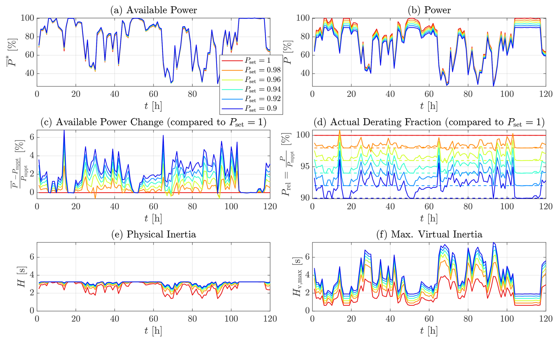
Figure 16 Simulation results at WF level for different derating power setpoints P_set based on the actual WF ambient wind data in Fig. 14.

Figure 17 shows the actual and forecasted $H_{\mathrm{v},max}$ values at WF level for exemplary power setpoints P_set=1 (panel a) and P_set=96 % (panel b), with the different wind input data for the wake model given by Fig. 14. The additional combined minimum (“Comb Min”) forecast in Fig. 17 uses the “Pro Min” and “Pro Max” forecasts. More precisely, the “Comb Min” forecast finds the minimum $H_{\mathrm{v},max}$ values within the forecasted local wind speed range $v_{\mathrm{w},\text{pro},\text{min}}\le v_{\mathrm{w}}\le v_{\mathrm{w},\text{pro},\text{max}}$ for each WT, where $v_{\mathrm{w},\text{pro},\text{min}}$ and $v_{\mathrm{w},\text{pro},\text{max}}$ are given by wake modeling with “Pro Min” and “Pro Max” forecast input data, respectively. Since $H_{\mathrm{v},max}$ is a nonlinear function of v_w for a given P_set, a nonlinear optimization algorithm solves $min{H}_{\mathrm{v},max}\left(v_{\mathrm{w}}\right)$ such that $v_{\mathrm{w},\text{pro},\text{min}}\le v_{\mathrm{w}}\le v_{\mathrm{w},\text{pro},\text{max}}$ for each WT. Again, the considered WF values are given by the mean values across all WTs. In Fig. 17a and b, the “Comb Min” and “Pro Max” forecasts are similar most of the time, but notable deviations occur especially during time intervals with lower wind speeds, which is in line with Fig. 11.

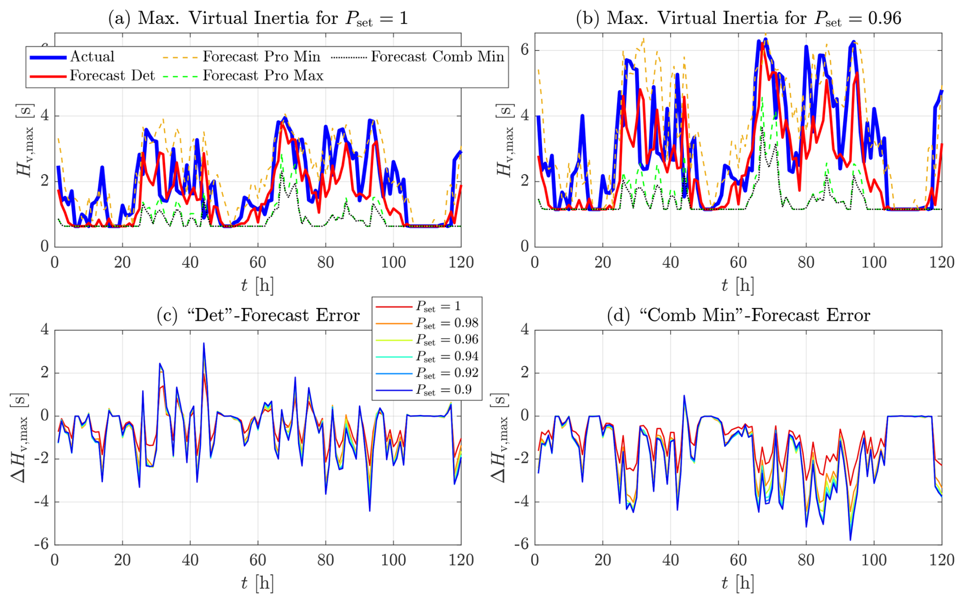
Figure 17 Comparison of actual and forecasted WF inertia, with errors (forecasted minus actual values) of the forecast types: deterministic (“Det”), probabilistic minimal (“Pro Min”), probabilistic maximal (“Pro Max”), and combined minimal (“Comb Min”).

Figure 17c and d show the “Det” and “Comb Min” inertia forecast errors for different derating. Due to lower $H_{\mathrm{v},max}$ variation for lower derating (see panels a, b), the absolute errors tend to be smaller in these cases. During almost all hours, the “Comb Min” forecast error is negative; i.e., the “Comb Min” forecast predicts a lower bound for $H_{\mathrm{v},max}$. This lower bound is especially relevant for (i) WF operators if they have to provide a minimum level of inertia or for (ii) system operators to analyze worst-case frequency events.

Figure 18 compares inertia monitoring errors due to simplified WF modeling for two variants: (i) replacing the numerical solution by the simplified solution (Sect. 3.4.2) of the optimization problem in Eq. (14) leads to the “Simple Opt” variant, and (ii) no-wake modeling leads to the “No-Wake” variant. Figure 18a–c consider the absolute error (“Abs. Error”) $\mathrm{\Delta }{H}_{\mathrm{v},max}$ (in s), and Fig. 18d–f consider the relative error (“Rel. Error”) $\mathrm{\Delta }{H}_{\mathrm{v},max}/H_{\mathrm{v},max}$ (in %). Both variants underestimate the WF inertia at all operating points, i.e., $\mathrm{\Delta }{H}_{\mathrm{v},max}=-\left|\mathrm{\Delta }{H}_{\mathrm{v},max}\right|$, such that the negative mean value (“−MEAN”) and the mean absolute error (MAE) are equal. The MAEs are 0.37 and 1.22 s (panel c) or 11.3 % and 38.5 % (panel f) for the “Simple Opt” and “No-Wake” variants, respectively. The error magnitude tends to increase with higher derating for the “Simple Opt” variant (see panels a, d), which is in line with the analysis at the WT level in Appendix J.

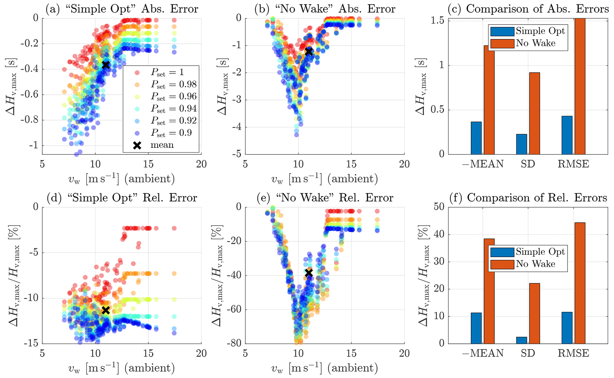
Figure 18 Inertia monitoring errors of the simplified optimization (“Simple Opt”) variant and the no-wake modeling (“No-Wake”) variant. For each considered variant and for each $P_{\text{set}}\in \mathit{\{}\mathrm{0.9},\mathrm{0.92},\mathrm{0.94},\mathrm{0.96},\mathrm{0.98},\mathrm{1}\mathit{\}}$, all 120 WF ambient wind data samples (one data point per hour) of the actual measurements in Fig. 14 are mapped to $H_{\mathrm{v},max}$ and to the corresponding errors (variant minus actual/proposed). The bars in panels (c) and (f) include all $\mathrm{6}\times \mathrm{120}=\mathrm{720}$ samples per variant, with the negative mean value (“−MEAN”) equal to the mean absolute error (MAE), sample standard deviation (“SD”), and root mean square error (RMSE).

In Fig. 19a and c, the WF inertia forecast error distributions of the “Simple Opt” and “No-Wake” variants are shifted to the left compared with the proposed variant due to the inertia underestimation in Fig. 18. At the samples with $\mathrm{\Delta }{H}_{\mathrm{v},max}>\mathrm{0}$ in Fig. 19a, the wind forecast errors overcompensate for the modeling errors $\mathrm{\Delta }{H}_{\mathrm{v},max}<\mathrm{0}$ in Fig. 18a. For the proposed complete numerical WF inertia forecasting, the MAE is 0.9 s or 26.8 %, as shown in Fig. 19b and d. For the “Simple Opt” forecasting, the MAE is 1.04 s or 30.3 %. For the “No-Wake” forecasting, the MAE is 1.68 s or 46.5 %. Thus, the simplified variants “Simple Opt” and “No Wake” increase the WF inertia forecasting MAE (in s) by $\frac{\mathrm{1.04}}{\mathrm{0.9}}-\mathrm{1}\approx \mathrm{16}\mathit{\%}$ and $\frac{\mathrm{1.68}}{\mathrm{0.9}}-\mathrm{1}\approx \mathrm{87}\mathit{\%}$, respectively.

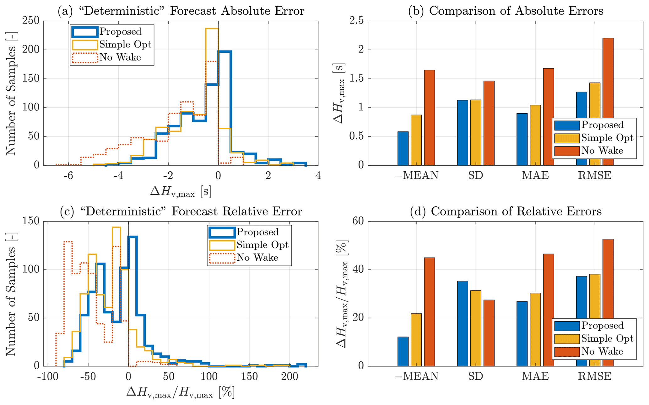
Figure 19 Inertia forecasting errors of the proposed (“Proposed”) and simplified variants (“Simple Opt”, “No Wake”). For each considered variant and for each $P_{\text{set}}\in \mathit{\{}\mathrm{0.9},\mathrm{0.92},\mathrm{0.94},\mathrm{0.96},\mathrm{0.98},\mathrm{1}\mathit{\}}$, all 120 WF ambient wind data samples (one data point per hour) of the deterministic (“Det”) forecast in Fig. 14 are mapped to $H_{\mathrm{v},max}$. Thus, the distributions shown include $\mathrm{6}\times \mathrm{120}=\mathrm{720}$ samples per variant, with negative mean value (“−MEAN”), sample standard deviation (“SD”), mean absolute error (MAE), and root mean square error (RMSE).

5 Conclusions

Grid-forming VSM control limits the initial ROCOF by inertia provision and thus enables grid frequency stability in future power systems with a high share of IBRs. VSM inertia can be adapted based on the required grid support. VSM control extracts WT kinetic energy reserve for inertia provision, but physical and virtual WT inertia differ in general. The WT with physical inertia constant H rotates asynchronously, whereas the VSM with virtual inertia constant H_v synchronizes with the grid frequency. However, in contrast to the grid-following control without inertia provision, the rotor speed and grid frequency dynamics are not completely decoupled anymore; i.e., the VSM requires the WT energy or power for grid synchronization. Thus, WT operating limits must be taken into account for proper grid synchronization with unsaturated inertia provision. Furthermore, the consideration of intra-farm turbine-to-turbine interactions is of great significance for a precise quantification of the inertia that can be provided to the grid. The participation in future inertia markets could be facilitated by short-term prediction of the maximum feasible inertia capability of the WF over varying inflow and operational conditions.

In contrast to existing solutions, the proposed formulation considers the WF grid-forming capability in terms of the maximum feasible inertia constant $H_{\mathrm{v},max}$ by simulating the inertial response of VSM-controlled WTs. Furthermore, the proposed formulation takes into account the intra-farm turbine-to-turbine interactions, as they have a large influence on the local wind condition at the turbines and have largely been ignored in the existing studies evaluating inertia provision capability. Under varying wind conditions, the derived simplified solution without dynamic WT simulations exhibits a trend similar to that of the complete numerical solution with dynamic WT simulations. However, the simplified solution significantly underestimates the optimal tuning value $H_{\mathrm{v}}=H_{\mathrm{v},max}$ for maximum inertia provision. In addition, the proposed dynamic WT simulations give deeper insights into the WT inertial response, including the relevance of operating limits and the interactions among different controllers, such as VSM control, MPPT compensation, MRS-based derating, active power droop control, and blade pitch control.

The proposed MRS-based derating increases the WT kinetic energy reserve for inertia provision with negligible impact on the thrust force. However, upon reaching the maximum rotor speed, further derating increases the pitch angle, significantly reducing thrust force and wake effects. Considering the aerodynamic trajectory of the power coefficient c_p(t) as a function of the tip ratio λ(t) during the inertial response to the worst-case ROCOF, the MRS-based derating provides kinetic energy and power headroom for inertia provision. This is achieved by initial operation with $\left(\mathit{\lambda }\right(t_{\mathrm{0}})>{\mathit{\lambda }}^{\star },c_{\mathrm{p}}(t_{\mathrm{0}})<c_{\mathrm{p}}^{\star })$ at the right side of the MPP $({\mathit{\lambda }}^{\star },c_{\mathrm{p}}^{\star })$; i.e., the power coefficient c_p(t) increases during WT deceleration. If the initial derating and thus the initial rotor speed Ω₀ are high enough, the rotor speed Ω(t) remains above its MPP value during the inertial response. In this case, no rotor speed recovery is required afterwards. The simulation results show that the proposed MRS-based derating increases the WF grid-forming capability in terms of $H_{\mathrm{v},max}$ over the complete wind speed range. For instance, considering a below-rated wind speed of $v_{\mathrm{w}}=\mathrm{9}\mathrm{m}{\mathrm{s}}^{-\mathrm{1}}$ in Sect. 4.2.2, a derating of 5 % significantly increases $H_{\mathrm{v},max}$ by ca. 68 %.

WT curtailment or derating increases the energy or power reserve for inertia provision, but wasting renewable energy should be avoided. Therefore, quantifying and forecasting inertia are essential for maximizing efficiency while ensuring grid stability. This paper demonstrated a generic approach for quantifying and forecasting the inertia provision of a WF based on weather forecasting, wake modeling, and mapping local WT operating points to grid-forming capabilities. The actual WF power loss is smaller than expected by local WT derating setpoints, since derating reduces wake effects and thus increases the available power. The $H_{\mathrm{v},max}$ forecast error depends on the uncertainty in the WF ambient wind forecast. Taking this into account, the proposed lower bound prediction for $H_{\mathrm{v},max}$ combines probabilistic minimal and maximal wind forecasts. Even for this conservative estimation, $H_{\mathrm{v},max}$ varies over time, and the WF can provide more inertia than at rated power during many hours. The proposed optimization of the WT inertial response avoids large errors due to (over)simplification.

Future work should validate the simulated WT inertial response based on a higher-fidelity model or using real measurements. Utilizing the presented simulation results for WF control is straightforward when operating all WTs with the same power setpoint P_set for derating. However, future work may also consider an optimal WF control that distributes individual P_set values to each WT, e.g., to maximize WF power while providing the desired inertia. Based on the new grid codes and inertia market requirements, the future mechanical and electrical designs of WTs and WFs should consider enhanced capabilities for grid-forming control, including inertia provision.

Appendix A: Nomenclature

D	Diameter
DFIM	Doubly fed induction machine
FCNN	Fully connected neural network
HVDC	High-voltage DC current
IBR	Inverter-based resource
LUT	Lookup table
MAE	Mean absolute error
MPP	Maximum power point
MPPT	Maximum power point tracking
MRS	Maximum rotation strategy
NWP	Numerical weather prediction
OP	Operating point
PGPE	Policy gradient with parameter-based exploration
RMSE	Root mean square error
ROCOF	Rate of change of frequency
SCR	Short-circuit ratio
SD	Standard deviation
SM	Synchronous machine
VSM	Virtual synchronous machine
WF	Wind farm
WT	Wind turbine

cp	Power coefficient
ct	Thrust coefficient
dt	Damping coefficient of tower spring–mass–damper system
D	Damping factor
ΔP	Power imbalance
Δt	Time duration
Ekin	Kinetic energy
f	Frequency
Ft	Aerodynamic thrust force
H	Inertia constant
ke	Electromagnetic feedback gain
kt	Stiffness coefficient of tower spring–mass–damper system
m	Torque
M	Non-dimensional torque
mt	Mass of tower spring–mass–damper system
n	Total number of turbines
${\stackrel{\mathrm{‾}}{c}}_{\mathrm{p}}$	Power coefficient corresponding to the available power
$\stackrel{\mathrm{‾}}{P}$	Non-dimensional available power
p	Power
P	Non-dimensional power
Pw	Power of the incoming wind
r	Radius of the rotor
s	Laplace-domain variable
st	Tower-top fore–aft displacement
t	Time variable
u	Voltage
$v_{\mathrm{w}}^u$	North-aligned component of the wind measurement
$v_{\mathrm{w}}^v$	East-aligned component of the wind measurement
vw	Wind speed
${\stackrel{\mathrm{̃}}{v}}_{\mathrm{w}}$	Relative wind speed
w	Weight variable
x	State variable

β	Blade pitch angle
δ	Load angle
ϵ	Threshold
λ	Tip-speed ratio
μ	Mean
ω	Angular frequency
ωn	Natural angular frequency of a second order system
Ω	Non-dimensional angular frequency
ϕ	Electrical angle
ρ	Air density
σ	Standard deviation
Θ	Moment of inertia
ζ	Damping ratio of a second order system

□comb	Value that combines min and max probabilistic forecasts
□d	Droop
□Det	Deterministic forecast value
□dp	Damping
□e	Electrical
□m	Mechanical
${\square }_{max}$	Maximum
□meas	Measured
${\square }_{min}$	Minimum
□mpp	Value at the maximum power point
□mppt	Value for maximum power point tracking
□R	Rated
□ref	Reference
□pu	Per unit value
□rec	Value for an additional WT rotor speed recovery constraint
□s	System/grid
□set	Setpoint
□pro	Probabilistic forecast value
□v	Virtual/ VSM
□0	Initial/steady-state value

□[i]	Value for ith turbine
${\square }^{\star }$	Optimal value
$\dot{\square }$	Time derivative $\mathrm{d}\square /\mathrm{d}t$

Appendix B: Grid impedance and electromagnetic feedback for VSM control

The grid impedance comprises several physical impedances, such as transformer or line impedances, but also include virtual impedances emulated by inverter control (Taul et al., 2020; VDE, 2024a). Moreover, for type 3 WTs, which use DFIMs, the physical grid impedance includes the DFIM stator impedance (Thommessen and Hackl, 2024). For type 4 WTs, which use full-scale back-to-back inverters, the physical grid impedance includes LC (L) filter impedances connected to the grid-side inverter (Taul et al., 2020). A high grid impedance (corresponding to a weak grid connection) leads to a lower electromagnetic feedback gain k_e (Thommessen and Hackl, 2024, Sect. III.E) and a lower natural angular velocity ω_n,v in Eq. (11), resulting in a lower inertial response time. In contrast, a higher grid voltage increases k_e and ω_n,v (VDE, 2024a).

From the perspective of system operators or grid stability, minimum k_e or ω_n,v values characterize the worst case in terms of a weak grid connection and a slow inertial response. For instance, the weak grid connection of (offshore) WFs is characterized by a typical short-circuit ratio SCR<2 (Ghimire et al., 2025). Thus, Ghimire et al. (2025) recommend an operating point sweep between maximum and minimum SCR for testing grid-forming capabilities and (load angle) stability analysis.

From the perspective of WF operators or WT protection, the worst case is characterized by maximum k_e or ω_n,v values due to fast inertial response with high torque rates. Accordingly, the considered worst-case analysis of the WT grid-forming capability should assume maximum k_e or ω_n,v values. Grid code requirements (VDE, 2024a) implicitly define an admissible k_e or ω_n,v value range by specifying lower and upper limits for the grid impedance and voltage.

Appendix C: VSM torque versus power synchronization

Replacing the torque with power quantities in Fig. 4 results in a power instead of a torque synchronization loop (Roscoe et al., 2020). However, the normalized VSM power and torque are approximately equal (see Eq. 12). For type 4 WTs with full-scale back-to-back inverters, the VSM-controlled grid-side inverter (approximately) outputs the VSM power (see Appendix D), which is in line with the proposed simplified representation. However, for type 3 WTs with DFIMs, the VSM control is not implemented at the grid-side inverter but at the machine-side inverter connected to the DFIM rotor (see Appendix E). Considering VSM torque synchronization, the DFIM emulates the VSM torque rather than the VSM power (see Appendix E). In this case, the WT inertial power response (quasi-steady-state value) depends on the DFIM or WT rotor speed Ω according to P_e=ΩM_e. Consequently, for type 3 WTs with VSM torque synchronization, it would be necessary to distinguish between (i) the VSM parameter H_v, representing the inertial torque response $\mathrm{\Delta }{M}_{\mathrm{e}}=M_{\mathrm{e},\mathrm{v}}\approx P_{\mathrm{v}}\approx -\mathrm{2}{H}_{\mathrm{v}}{\dot{\mathrm{\Omega }}}_{\mathrm{s}}$ (see also Eq. 12), and (ii) a power-equivalent inertia constant H_eq for inertia provision, representing the inertial power response (e.g., $\mathrm{\Delta }{P}_{\mathrm{e}}\approx \mathrm{\Delta }{M}_{\mathrm{e}}\mathrm{\Omega }=:-\mathrm{2}{H}_{\text{eq}}{\dot{\mathrm{\Omega }}}_{\mathrm{s}}$, with $\mathrm{\Omega }\ne {\mathrm{\Omega }}_{\mathrm{s}}\approx \mathrm{1}$ in general). In contrast, for type 4 WTs, H_v defines the inertial power response of both WTs and VSMs, i.e., $\mathrm{\Delta }{P}_{\mathrm{e}}=P_{\mathrm{v}}\approx -\mathrm{2}{H}_{\mathrm{v}}{\dot{\mathrm{\Omega }}}_{\mathrm{s}}$, and no additional definition of H_eq is needed for quantifying inertia provision.

For simplicity, this paper considers type 4 WTs, for which torque and power synchronization loops result in similar inertial responses. For type 3 WTs with torque synchronization, the proposed generic approach is also applicable by taking H_eq≠H_v into account. In this case, the VSM representation in Fig. 2 must simply be adjusted by redefining the VSM power in Eq. (10) as $P_{\mathrm{v}}:=\mathrm{\Omega }{M}_{\mathrm{e},\mathrm{v}}$. For type 3 WTs with power synchronization, it must simply be taken into account that the VSM synchronization speed ω_n,v depends on the DFIM speed (see Appendix E).

Appendix D: VSM control for type 4 WTs and assumptions

For type 4 WTs based on full-scale back-to-back inverters, the grid-side and machine-side inverters are connected via a DC link. The grid-side inverter tracks the WT power reference based on VSM control, whereas the machine-side inverter controls the DC-link voltage u_dc (Roscoe et al., 2020; Meseguer Urban et al., 2019; Nguyen et al., 2022). Strictly speaking, the power of the machine-side and grid-side inverter is not equal during u_dc transients due to the DC-link buffer energy $E_{\text{dc}}=\frac{\mathrm{1}}{\mathrm{2}}{C}_{\text{dc}}{u}_{\text{dc}}^{\mathrm{2}}$ with DC-link capacity C_dc. However, E_dc is usually negligible in comparison with the WT kinetic energy reserve (i.e., E_dc≪E_kin); see also Hackl et al. (2018). Thus, E_dc is usually not relevant for inertia provision. Moreover, a small E_dc requires a fast-reacting or aggressively tuned DC-link voltage control to keep u_dc within its small admissible voltage range (Thommessen and Hackl, 2024). Thus, this paper neglects the power difference or delay between machine-side and grid-side inverters.

Appendix E: VSM control for type 3 WTs and assumptions

For type 3 WT based on DFIMs, the directly grid-connected DFIM stator generates most of the power. The DFIM rotor is connected to the grid via back-to-back inverters, with the power flow depending on the DFIM slip Ω−Ω_s (Dirscherl and Hackl, 2016). With the VSM torque defined as the DFIM torque (i.e., $M_{\mathrm{e},\mathrm{v}}:=M_{\mathrm{e}}$), the DFIM stator power approximately equals the VSM power (i.e., $P_{\text{stator}}={\mathrm{\Omega }}_{\mathrm{s}}{M}_{\mathrm{e}}\approx P_{\mathrm{v}}$) (Rodriguez-Amenedo et al., 2021; Thommessen and Hackl, 2024). However, the total electrical DFIM power includes the DFIM rotor power as well; i.e., $P_{\mathrm{e}}=P_{\text{stator}}+P_{\text{rotor}}={\mathrm{\Omega }}_{\mathrm{s}}{M}_{\mathrm{e}}+\left(\mathrm{\Omega }-{\mathrm{\Omega }}_{\mathrm{s}}\right)M_{\mathrm{e}}=\mathrm{\Omega }{M}_{\mathrm{e}}\ne P_{\mathrm{v}}$ (Dirscherl and Hackl, 2016). Alternatively, Shah and Gevorgian (2020) propose grid-forming control for DFIMs based on a power instead of a torque synchronization loop with a power feedback P_v:=P_e instead of a torque feedback $M_{\mathrm{e},\mathrm{v}}:=M_{\mathrm{e}}$. In this case, the DFIM electrical power feedback gain k_e varies with the WT rotor speed Ω according to P_e=ΩM_e, and thus the VSM inertial response time or ω_n,v in Eq. (11) also varies.

Appendix F: Prioritization of inertia provision over droop control

Both the inertial response and the droop control are essential for grid frequency stability. Firstly, the inertial response is always needed to limit the magnitude of ROCOF regardless of its sign, i.e., even during frequency recovery. Otherwise, if the ROCOF is too high, grid-connected resources trip, e.g., due to loss of synchronism or load angle instability. Secondly, active power droop control (or primary frequency control) is needed to limit the steady-state frequency deviation. Although WTs can reduce their power to support over-frequency events, WTs in MPPT mode cannot permanently increase their power for prolonged support of under-frequency events. Thus, droop control has to increase the WT output power only if quasi-steady power reserves are available due to previous derating (VDE, 2024a). A temporary droop control activation, i.e., a temporary power offset proportional to the frequency deviation based on kinetic energy extraction, is often proposed for a fast frequency response of grid-following WTs (Godin et al., 2019; Lee et al., 2016). Although this would temporarily increase frequency support, the slower frequency response would hide the urgency of power adaptation for grid support from other grid-connected resources, thereby delaying or decreasing their response. This may also lead to a secondary frequency event after the temporary support. Thus, such a temporary droop control activation is not considered in the German grid code for grid-forming technologies (VDE, 2024a), nor is it considered in this work.

In summary, the inertial response limits the ROCOF, which determines the time available to react, e.g., for protection devices to shed loads or for other resources to ramp up power production. Thus, the inertial response has the highest priority and uses all power reserves, including kinetic energy. With increasing frequency deviation, droop control (or primary frequency control) limits steady-state frequency deviation. For under-frequency events, droop control is only feasible for WTs if wind power reserves are available due to previous derating. WTs should not use kinetic energy reserves for temporary droop control activation in order to properly communicate the droop power demand to other resources via the grid frequency.

Appendix G: WT rotor speed recovery and requirements

Assuming initial operation at the maximum power point (MPP), the WT deceleration during the inertial response decreases the aerodynamic power. For the example shown in Sect. 4, this is illustrated by the plot shown in Fig. 9. Thus, during the so-called recovery phase after the frequency event, the output power has to decrease below the initial power to maintain speed. In fact, the WT power is reduced even further to (slowly) re-accelerate the rotor, which affects the grid frequency recovery and may lead to a secondary frequency drop (Bao et al., 2016; Duckwitz, 2019; Höhn et al., 2024). Thus, a former draft of the German grid code (VDE, 2024a, version 0.1) explicitly prohibited reducing the output power for speed recovery. With reference to the example considered in this work, reducing the output power below its initial value to re-accelerate the rotor would not be allowed after the ROCOF returns to zero at t=4 s in Fig. 9.

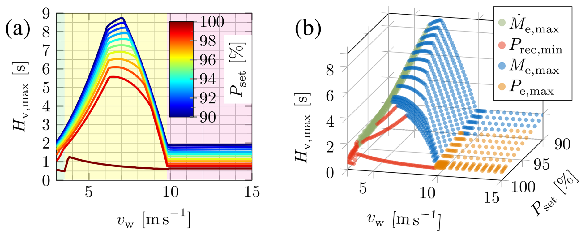
Figure G1 Proposed solution with additional recovery power constraint: maximum virtual inertia constant for different operating points (v_w,P_set) and with active optimization constraints highlighted in panel (b).

However, this constraint is probably more restrictive than necessary. In fact, the frequency event defined in the grid code (VDE, 2024b) may not represent a realistic situation but can be regarded as a worst-case test to verify the inertia provision capability of a grid-connected unit. Godin et al. (2019) consider a frequency event with less severe ROCOFs, which requires a lower power increase ΔP over a longer period Δt, before reaching the frequency nadir. However, the kinetic energy extraction ΔPΔt may be similar to the one used in our work. Although Godin et al. (2019) assume a slower frequency recovery afterwards, the rotor speed recovery is similar, since speed recovery takes much longer than frequency recovery (see Fig. 9). Considering the power reduction due to MPP deviations during the recovery phase of a real WF, Godin et al. (2019) observe that similar reductions can be expected simply from changes in wind conditions. Moreover, the inertial response superimposes all variations in WT operating points, which, in reality, results in a smoothing effect on the grid frequency during the recovery phase (see also Thommessen and Hackl, 2024). Consequently, requirements for power recovery should not be too restrictive. As per the recent version of the German grid code (VDE, 2024a), no recovery power constraints are considered in this paper by default, although they can be easily included if necessary, as demonstrated next.

The optimization results in Fig. G1 include an additional constraint for the recovery phase after the WT inertial response. More precisely, the power P_mppt – available for rotor speed recovery after the frequency event ends at t_end:=4.1 s – is not allowed to fall more than 1 % below the initial power; i.e., $P_{\text{rec},min}:=P_{\mathrm{m},\mathrm{0}}-\mathrm{1}\mathit{\%}\le P_{\text{mppt}}\left(\mathrm{\Omega }\right(t_{\text{end}}\left)\right)$. This $P_{\text{rec},min}$ constraint significantly limits the inertia provision at below-rated wind speeds for low derating, since most of the WT kinetic energy reserve cannot be used. In this case, the WT rotor speed limit Ω_min is irrelevant, as the $P_{\text{rec},min}$ constraint is active instead.

Appendix H: Simplified torque rate constraint

Limiting the torque rate ${\dot{M}}_{\mathrm{e}}$ in Eq. (14) contradicts the simplifying assumption of an ideal power pulse in Eq. (17) with infinite torque rate. However, instead of neglecting the actual limit ${\dot{M}}_{\mathrm{e},max}$, a simplified torque rate constraint can be derived as follows. Transforming Eq. (11) in the time domain, the VSM torque response to a ROCOF step change from zero to ${\dot{\mathrm{\Omega }}}_{\mathrm{s}}$ is given by

$$\begin{array}{}\text{(H1)}& M_{\mathrm{e},\mathrm{v}}\left(t\right)={\dot{\mathrm{\Omega }}}_{\mathrm{s}}{\displaystyle \frac{\mathrm{4}{H}_{\mathrm{v}}+D_{\mathrm{v}}t}{\mathrm{2}}}{e}^{-\frac{D_{\mathrm{v}}}{\mathrm{4}{H}_{\mathrm{v}}}t}-\mathrm{2}{H}_{\mathrm{v}}{\dot{\mathrm{\Omega }}}_{\mathrm{s}}.\end{array}$$

By differentiating with respect to time, one gets

$$\begin{array}{}\text{(H2)}& {\dot{M}}_{\mathrm{e},\mathrm{v}}\left(t\right)=-{\dot{\mathrm{\Omega }}}_{\mathrm{s}}{\displaystyle \frac{{D_{\mathrm{v}}}^{\mathrm{2}}t}{\mathrm{8}{H}_{\mathrm{v}}}}{e}^{-\frac{D_{\mathrm{v}}}{\mathrm{4}{H}_{\mathrm{v}}}t},\end{array}$$

and

$$\begin{array}{}\text{(H3)}& {\ddot{M}}_{\mathrm{e},\mathrm{v}}\left(t\right)=-{\dot{\mathrm{\Omega }}}_{\mathrm{s}}{\displaystyle \frac{{D_{\mathrm{v}}}^{\mathrm{2}}}{\mathrm{8}{H}_{\mathrm{v}}}}\left(\mathrm{1}-{\displaystyle \frac{D_{\mathrm{v}}}{\mathrm{4}{H}_{\mathrm{v}}}}t\right)e^{-\frac{D_{\mathrm{v}}}{\mathrm{4}{H}_{\mathrm{v}}}t}.\end{array}$$

Zeroing Eq. (H3) and inserting the solution into Eq. (H2) yield the maximum VSM torque rate

$$\begin{array}{}\text{(H4)}& max{\dot{M}}_{\mathrm{e},\mathrm{v}}\left(t\right)={\dot{M}}_{\mathrm{e},\mathrm{v}}\left(t={\displaystyle \frac{\mathrm{4}{H}_{\mathrm{v}}}{D_{\mathrm{v}}}}\right)=-{\displaystyle \frac{\mathrm{1}}{\mathrm{2}e}}{\dot{\mathrm{\Omega }}}_{\mathrm{s}}{D}_{\mathrm{v}}.\end{array}$$

Neglecting the WT deceleration until reaching the maximum torque rate, i.e., Ω(t)≈Ω₀, and scaling Eq. (H4) by $\mathrm{1}/{\mathrm{\Omega }}_{\mathrm{0}}$ due to asynchronous WT rotation with respect to VSM speed or grid frequency, the simplified WT torque rate constraint is given by

$$\begin{array}{}\text{(H5)}& max{\dot{M}}_{\mathrm{e}}={\displaystyle \frac{max{\dot{M}}_{\mathrm{e},\mathrm{v}}}{{\mathrm{\Omega }}_{\mathrm{0}}}}={\displaystyle \frac{{\dot{\mathrm{\Omega }}}_{\mathrm{s},max}}{\mathrm{2}e{\mathrm{\Omega }}_{\mathrm{0}}}}{D}_{\mathrm{v}}\left(H_{\mathrm{v}}\right)\le {\dot{M}}_{\mathrm{e},max}.\end{array}$$

Appendix I: Steady-state calculation

Solving the optimization problem in Eq. (14) for a given WT operating point defined by (v_w,P_set) requires initializing the simulation model to a steady state. However, the steady-state conditions are unknown in general. Instead of running time-consuming simulations until reaching steady state, an alternative is proposed to speed up the optimization. At the equilibrium point, mechanical and electrical power are equal; i.e., the initial steady states (Ω₀,β₀) solve the minimization problem

$$\begin{array}{}\text{(I1)}& ({\mathrm{\Omega }}_{\mathrm{0}},{\mathit{\beta }}_{\mathrm{0}}):=\text{arg}min\left|e\right(\mathrm{\Omega },\mathit{\beta }\left)\right|,\end{array}$$

where $e(\mathrm{\Omega },\mathit{\beta }):=P_{\mathrm{m}}-P_{\mathrm{e}}=P_{\mathrm{w}}\left(v_{\mathrm{w}}\right)c_{\mathrm{p}}(\mathrm{\Omega },\mathit{\beta },v_{\mathrm{w}})-\mathrm{\Omega }{M}_{\mathrm{e}}(\mathrm{\Omega },v_{\mathrm{w}},P_{\text{set}})=\mathrm{0}$.

The following analysis evaluates (v_w,P_set) and identifies active constraints in the different WT operating regions to convert Eq. (I1) into simpler one-dimensional subproblems.

Firstly, for MPPT with P_set=1 and M_e=M_mppt, Eq. (I1) can be rewritten as (Thommessen and Hackl, 2024)

$$\begin{array}{}\text{(I2)}& \begin{array}{rl}& \left({\stackrel{\mathrm{‾}}{\mathrm{\Omega }}}^{\star },{\stackrel{\mathrm{‾}}{\mathit{\beta }}}^{\star }\right):=\text{arg}min\left|{\stackrel{\mathrm{‾}}{e}}^{\star }\right(\mathrm{\Omega },\mathit{\beta }\left)\right|\\ & \text{s.t.}\left\{\begin{array}{l}{\mathrm{\Omega }}_{min}\le \mathrm{\Omega }\le \mathrm{1},\\ {\mathit{\beta }}_{min}\le \mathit{\beta }\le {\mathit{\beta }}_{max},\\ {\mathit{\beta }}_{min}=\mathit{\beta }\text{if}{v}_{\mathrm{w}}\le v_{\mathrm{w},\mathrm{R}},\\ \mathrm{\Omega }=\mathrm{1}\text{if}{v}_{\mathrm{w}}>v_{\mathrm{w},\mathrm{R}},\end{array}\right.\end{array}\end{array}$$

where ${\stackrel{\mathrm{‾}}{e}}^{\star }(\mathrm{\Omega },\mathit{\beta }):=P_{\mathrm{m}}-\mathrm{\Omega }{M}_{\mathrm{e}}=P_{\mathrm{w}}{c}_{\mathrm{p}}-\mathrm{\Omega }{M}_{\text{mppt}}$, for a given wind speed v_w. One-dimensional optimizations are solved for the following problems:

$$\begin{array}{}\text{(I3)}& \left\{\begin{array}{ll}{v}_{\mathrm{w},\text{cut-in}}\le v_{\mathrm{w}}<v_{\mathrm{w},\text{II},min}& \Rightarrow \left(\begin{array}{l}{\stackrel{\mathrm{‾}}{\mathrm{\Omega }}}^{\star }\\ {\stackrel{\mathrm{‾}}{\mathit{\beta }}}^{\star }\end{array}\right)=\left(\begin{array}{l}\text{arg}min\left|{\stackrel{\mathrm{‾}}{e}}^{\star }\right|\\ {\mathit{\beta }}_{min}={\mathit{\beta }}_{min}\left(\mathit{\lambda }\right)\end{array}\right),\\ v_{\mathrm{w},\text{II},min}\le v_{\mathrm{w}}\le v_{\mathrm{w},\mathrm{R}}& \Rightarrow \left(\begin{array}{l}{\stackrel{\mathrm{‾}}{\mathrm{\Omega }}}^{\star }\\ {\stackrel{\mathrm{‾}}{\mathit{\beta }}}^{\star }\end{array}\right)=\left(\begin{array}{l}{\mathit{\lambda }}^{\star }\frac{v_{\mathrm{w}}}{{\mathit{\omega }}_{\mathrm{R}}r}\\ {\mathit{\beta }}_{min}={\mathit{\beta }}^{\star }\end{array}\right),\\ v_{\mathrm{w},\mathrm{R}}<v_{\mathrm{w}}\le v_{\mathrm{w},\text{cut-out}}& \Rightarrow \left(\begin{array}{l}{\stackrel{\mathrm{‾}}{\mathrm{\Omega }}}^{\star }\\ {\stackrel{\mathrm{‾}}{\mathit{\beta }}}^{\star }\end{array}\right)=\left(\begin{array}{l}\mathrm{1}\\ \text{arg}min\left|{\stackrel{\mathrm{‾}}{e}}^{\star }\right|\end{array}\right),\end{array}\right.\end{array}$$

with either ${\stackrel{\mathrm{‾}}{\mathrm{\Omega }}}^{\star }$ or ${\stackrel{\mathrm{‾}}{\mathit{\beta }}}^{\star }$ known in advance (except for the transition region I–II in the first case, where ${\stackrel{\mathrm{‾}}{\mathit{\beta }}}^{\star }={\mathit{\beta }}_{min}\left(\mathit{\lambda }\right)$ is calculated based on $\mathit{\lambda }={\stackrel{\mathrm{‾}}{\mathrm{\Omega }}}^{\star }{\mathit{\omega }}_{\mathrm{R}}r/v_{\mathrm{w}}$). For the available WT power ${\stackrel{\mathrm{‾}}{P}}^{\star }$ in Eq. (7), the MPPT power coefficient is given by Eq. (8) with $({\stackrel{\mathrm{‾}}{\mathrm{\Omega }}}^{\star },{\stackrel{\mathrm{‾}}{\mathit{\beta }}}^{\star })$ given by Eq. (I3).

Secondly, to derate with P_set<1 and $P_{\mathrm{e}}={\stackrel{\mathrm{‾}}{P}}^{\star }{P}_{\text{set}}$, Eq. (I1) can be rewritten as

$$\begin{array}{}\text{(I4)}& ({\mathrm{\Omega }}_{\mathrm{0}},{\mathit{\beta }}_{\mathrm{0}}):=\text{arg}min\left|\stackrel{\mathrm{̃}}{e}\right(\mathrm{\Omega },\mathit{\beta }\left)\right|,\end{array}$$

where $\stackrel{\mathrm{̃}}{e}(\mathrm{\Omega },\mathit{\beta }):=P_{\mathrm{m}}-P_{\mathrm{e}}=P_{\mathrm{w}}{c}_{\mathrm{p}}-{\stackrel{\mathrm{‾}}{P}}^{\star }{P}_{\text{set}}$, which is solved in two substeps. In the first substep, ignoring the speed limit by assuming inactive pitch control leads to the theoretical steady-state rotor speed

$$\begin{array}{}\text{(I5)}& {\stackrel{\mathrm{̃}}{\mathrm{\Omega }}}_{\mathrm{0}}:=\text{arg}min\left|\stackrel{\mathrm{̃}}{e}\right(\mathrm{\Omega },\mathit{\beta }={\mathit{\beta }}_{min}\left)\right|,\end{array}$$

with ${\mathit{\beta }}_{min}={\mathit{\beta }}_{min}\left(\mathit{\lambda }\right)$. The second substep takes the speed limit Ω=1 into account; i.e.,

$$\begin{array}{}\text{(I6)}& \Rightarrow \left\{\begin{array}{l}{\stackrel{\mathrm{̃}}{\mathrm{\Omega }}}_{\mathrm{0}}\le \mathrm{1}\Rightarrow \left(\begin{array}{c}{\mathrm{\Omega }}_{\mathrm{0}}\\ {\mathit{\beta }}_{\mathrm{0}}\end{array}\right)=\left(\begin{array}{c}{\stackrel{\mathrm{̃}}{\mathrm{\Omega }}}_{\mathrm{0}}\\ {\mathit{\beta }}_{min}\end{array}\right)\\ {\stackrel{\mathrm{̃}}{\mathrm{\Omega }}}_{\mathrm{0}}>\mathrm{1}\Rightarrow \left(\begin{array}{c}{\mathrm{\Omega }}_{\mathrm{0}}\\ {\mathit{\beta }}_{\mathrm{0}}\end{array}\right)=\left(\begin{array}{c}\mathrm{1}\\ \text{arg}min\left|\stackrel{\mathrm{̃}}{e}\right|\end{array}\right).\end{array}\right.\end{array}$$

This way, the original two-dimensional optimization problem given by Eq. (I1) has been converted into the simpler one-dimensional subproblems Eqs. (I3), (I5), and (I6).

Appendix J: Results of the simplified solution for maximum inertia provision

The results of the simplified solution derived in Sect. 3.4.2 are shown in the left plot of Fig. J1. In comparison with the results of the complete numerical solution in Fig. 11, the simplified solution underestimates the WT inertia provision capability. Considering the right plot of Fig. J1, significant simplification errors can be observed; e.g., $\left|\mathrm{\Delta }{H}_{\mathrm{v},max}\right|>\mathrm{1}\mathrm{s}$ at $v_{\mathrm{w}}=\mathrm{7}\mathrm{m}{\mathrm{s}}^{-\mathrm{1}}$ for P_set≤96 %. For P_set=1, one reason for the underestimation is that the simplified solution assumes a constant electrical power in Eq. (17), whereas in reality, the VSM inertial power P_v decreases with Ω_v≈Ω_s in Eq. (10). The underestimation significantly increases with higher derating, since the simplified solution only considers kinetic energy reserve and does not account for wind power reserve or changing aerodynamics. More precisely, the MRS-based derating leads to initial operation at the right side of the MPP. During the inertial response, the decreasing λ in combination with decreasing β increases the aerodynamic or mechanical power, which counteracts the WT rotor deceleration, as also shown in Fig. 10.

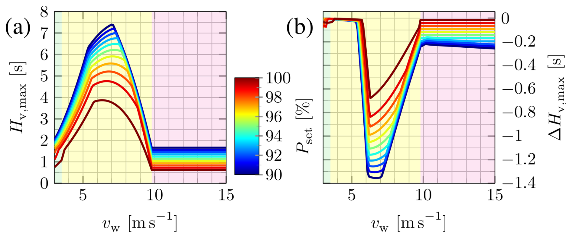
Figure J1 Simplified solution: maximum virtual inertia constant for different operating points (a) and simplification error or deviation from the complete numerical solution (b).

Appendix K: Further definitions and parameters

The inertial response time interval for evaluating extreme WT operating points in Figs. 12 and 13 is defined as

$$\begin{array}{}\text{(K1)}& \begin{array}{rl}& t_{\mathrm{0}}\le t\le min\mathit{\{}{t}_{\mathrm{1}},t_{\mathrm{2}}\mathit{\}},t_{\mathrm{1}}:=max\left\{t_{\mathrm{s},min},\text{arg}min\mathrm{\Omega }\left(t\right)\right\},\\ & t_{\mathrm{2}}:=\left\{\begin{array}{l}{t}_{\mathrm{1}},\text{if}\forall t\ge t_{\mathrm{0}}:{\stackrel{\mathrm{‾}}{P}}_{\mathrm{d}}\left(t\right)\le \mathrm{0},\\ mint\text{s.t.}{\stackrel{\mathrm{‾}}{P}}_{\mathrm{d}}\left(t\right)>\mathrm{0}\wedge t\ge t_{\mathrm{s},min},\text{otherwise}\end{array}\right\},\end{array}\end{array}$$

where t₁ takes into account that the WT speed nadir may occur (shortly) after the grid frequency nadir at $t_{\mathrm{s},min}$, and t₂ takes into account that the droop control may cause further uncritical WT deceleration for $t\ge t_{\mathrm{s},min}$.