the Creative Commons Attribution 4.0 License.
the Creative Commons Attribution 4.0 License.
 | 25 Aug 2020
Aeroelastic load validation in wake conditions using nacelle-mounted lidar measurements
Nikolay Dimitrov
Alfredo Peña
We propose a method for carrying out wind turbine load validation in wake conditions using measurements from forward-looking nacelle lidars. Two lidars, a pulsed- and a continuous-wave system, were installed on the nacelle of a 2.3 MW wind turbine operating in free-, partial-, and full-wake conditions. The turbine is placed within a straight row of turbines with a spacing of 5.2 rotor diameters, and wake disturbances are present for two opposite wind direction sectors. The wake flow fields are described by lidar-estimated wind field characteristics, which are commonly used as inputs for load simulations, without employing wake deficit models. These include mean wind speed, turbulence intensity, vertical and horizontal shear, yaw error, and turbulence-spectra parameters. We assess the uncertainty of lidar-based load predictions against wind turbine on-board sensors in wake conditions and compare it with the uncertainty of lidar-based load predictions against sensor data in free wind. Compared to the free-wind case, the simulations in wake conditions lead to increased relative errors (4 %–11 %). It is demonstrated that the mean wind speed, turbulence intensity, and turbulence length scale have a significant impact on the predictions. Finally, the experiences from this study indicate that characterizing turbulence inside the wake as well as defining a wind deficit model are the most challenging aspects of lidar-based load validation in wake conditions.
- Article
(6590 KB) - Full-text XML
- BibTeX
- EndNote


Wind turbines are designed according to reference wind conditions described in the IEC standards (IEC, 2019). These reference conditions are used to establish the full design load basis and for the purpose of certification of turbine designs. Nevertheless, certified turbines need to be further verified to withstand the site-specific loads during the entire lifetime, when site conditions exceed those of the type certified. As a current best practice, the wind turbine (WT) operating loads are predicted using high-fidelity aeroelastic simulations based on site-specific environmental conditions. The environmental conditions are typically obtained from anemometers installed on meteorological masts in the proximity of the wind turbine location. These mast measurements, and therefore the uncertainty quantification of the aeroelastic model, are usually limited to wake-free sectors. However, wind conditions inside wind farms are significantly different than those in undisturbed wind conditions (Frandsen, 2007).
Wake effects are responsible for wind speed reduction and turbulence level increase, generally resulting in reduced power productions and increased load levels (Larsen et al., 2013). To account for these effects, aeroelastic load simulations are combined with wake models, which predict wake-induced effects on the flow field approaching individual WTs. The most applied approach consists of increasing the turbulence in load simulations, resulting in a load increase which should correspond to the effect of the wake-added turbulence. The effective turbulence depends on the park layout and on the material properties of the turbine components under consideration (Frandsen, 2007). This approach is recommended by the IEC61400-1. An alternative and more detailed practice also described in the IEC standard relies on the use of the dynamic wake meandering (DWM) model (Larsen et al., 2006, 2007; Madsen et al., 2010), which is an engineering model providing simulated wind field time series including wake deficits.
The comparison of fatigue loads predicted using the DWM model and the effective turbulence approach by the IEC showed a discrepancy of 20 % (Thomsen et al., 2007). The uncertainty varied according to the inflow conditions and spacing between turbines. The work of Larsen et al. (2013) showed a very fine agreement between both power and load measurements and predictions based on a site-specific calibrated DWM model for the Dutch Egmond aan Zee wind farm. However, the study did not quantify uncertainty in a systematic approach. More recently, Reinwardt et al. (2018) estimated fatigue load biases in the range 11 %–15 % for the tower bottom and 8 %–21 % for the blade-root flapwise bending moments using the DWM model. To date, these approaches are characterized by a significant level of uncertainty, due to the stochastic nature of environmental conditions and the various simplifying assumptions used in the wake model definitions (Schmidt et al., 2011). Further, these results motivate the need for improving wind turbine load validation approaches in wake conditions.
The recent applications of lidars in the wind energy field demonstrate the feasibility of these systems to reconstruct inflow wind conditions including mean wind speed (Raach et al., 2014; Borraccino et al., 2017), turbulence (Mann et al., 2009; Branlard et al., 2013; Peña et al., 2017; Newman and Clifton, 2017), and wake characteristics (Bingöl et al., 2010; Iungo and Porté-Agel, 2014; Machefaux et al., 2016), among others. Nacelle-mounted lidars enable us to measure wind field characteristics for any wind direction/nacelle yaw position, including situations when the turbine rotor is in the wake of a neighbouring turbine. An excellent level of agreement has been found between the nacelle-mounted lidar-estimated and mast-measured mean wind speed in free-wind conditions (Borraccino et al., 2017). Power curve validations using nacelle-mounted lidars have been showing promising results (Wagner et al., 2014). Although lidar-derived along-wind variances could deviate from those derived from cup anemometer measurements (Peña et al., 2017), the load predictions in wake-free sectors based on nacelle-lidar wind field representations resulted in uncertainties lower than or equal to those obtained with mast measurements (Dimitrov et al., 2019).
Based on these findings, we extend the load validation procedure defined in Dimitrov et al. (2019) to include wake conditions. Therefore, wake-induced effects are accounted for by means of wind field parameters commonly used as inputs for load simulations, which are reconstructed using lidar measurements, yet without employing wake deficit models. The objective of this study is to demonstrate how loads in wake conditions can be predicted accurately, quantify the uncertainty, and compare it to the uncertainty of lidar-based load assessments in free wind. The further development of lidar-based load and power validation procedures can potentially replace the use of expensive meteorological masts in measurement campaigns as well as improve the wake field reconstruction for aeroelastic load simulations.
The paper is structured as follows. In Sect. 2, we introduce the requirements for load validation and describe the measurement campaign. In Sect. 3, we present the methods implemented to derive the wind field parameters for aeroelastic simulations and a wake detection algorithm. The results are provided in Sect. 4. First, we show the wake-induced effects on the lidar-estimated wind field parameters in Sect. 4.1 and 4.2. Then, we derive the wind field characteristics used as input for load simulations in Sect. 4.3. The uncertainties of load predictions are quantified in Sect. 4.4. The sensitivity of inflow parameters on load predictions and the uncertainty distribution of selected cases are assessed in Sect. 4.5. Finally, we discuss the findings and provide conclusions in the last two sections.
2.1 Requirements for load validation in wakes
The design load cases and load validation procedure for wind turbines are described in the IEC standards. The IEC61400-1 requires the evaluation of fatigue and extreme loading conditions induced by wake effects originating from neighbouring wind turbines. The increase in loading due to wake effects can be accounted for by the use of an added turbulence model, or by using more detailed wake models (i.e. DWM). Load validation guidelines are described in IEC61400-13 (IEC, 2015), which recommends the so-called one-to-one comparison, among a few approaches. This approach consists of carrying out individual aeroelastic simulations for each measured realization of environmental conditions. To date, wind conditions are obtained from meteorological masts.
The objective of this work is to carry out load validation of wind turbines operating in wake conditions using measurements from nacelle-mounted lidars only. The wake-induced effects are accounted for by lidar-estimated wind field characteristics, without employing wake deficit models. This implies that wake flow fields can be described by means of average flow characteristics commonly used as inputs for load simulations. We assess the viability of the suggested approach by carrying out a load validation study as follows:
-
one-to-one load comparison between measured and predicted load realizations using wind field characteristics derived from lidar measurements of the wake flow field;
-
uncertainty quantification in terms of the statistical properties of the ratios between measured and predicted load realizations;
-
comparison of lidar-based load prediction uncertainties in wakes against uncertainties of load predictions in free-wind conditions using lidar measurements.
We assume that the observed deviations in load predictions between those that are lidar-based under wake conditions and those that are lidar-based under free-wind conditions are solely due to the error in the wind field representation. This is a simplistic but conservative assumption, as the uncertainties of load predictions are a combination of uncertainty in the reconstructed wind profiles, aeroelastic model uncertainty, load measurement uncertainty, and statistical uncertainty (Dimitrov et al., 2019).
2.2 Measurement campaign
Wind and load measurements are collected from an experiment conducted at the Nørrekær Enge (NKE) wind farm during a period of 7 months between 2015 and 2016. The farm is located in the north-west of Denmark and consists of 13 Siemens 2.3 MW turbines, with a 93 m rotor diameter (D) and hub height of 80 m a.g.l. (above ground level). The turbines are installed in a single row oriented along the 75 and 255∘ direction compared to true north, with 487 m (5.2 D) spacing, as pictured in Fig. 1. The wind farm is located over flat terrain, and the surface is characterized by a mix between croplands and grasslands, and a fjord to the north (Peña et al., 2017). The prevailing wind direction is west (Borraccino et al., 2017).
The wind turbine T04 was instrumented with sensors for load measurements at the roots of two blades, tower top, and tower bottom (Vignaroli and Kock, 2016). The strain gauges were installed at 1.5 m from the blade-root flange, at 11.85 m below the lower surface of the tower top flange, and at 5.9 m above the upper surface of the tower bottom flange. The data acquisition software was set to sample at 35 Hz on all channels. Additional data were provided by the supervisory control and data acquisition (SCADA) system including nacelle wind speed and orientation, power output, blade pitch angles, and generator speed. A meteorological mast was installed at 232 m (2.5 D) distance from T04 in the direction of 103∘. The mast instrumentation comprises cup and sonic anemometers, wind vanes, and thermometers mounted at several heights, among others. Details about the instrumentations can be found in Vignaroli and Kock (2016) and Borraccino et al. (2017).
This study uses wind measurements from the cup anemometers at 57.5 and 80 m, which are used to derive wind speed, turbulence, and shear as discussed in the following sections. According to the definition in IEC61400-12-1 (IEC, 2017), the wake-free sector spans approximately 123∘ to 220∘. A narrow sector of 12∘ from 97 to 109∘ is chosen as free-wind reference to ensure close correspondence between lidar- and mast-measured parameters. Based on the farm geometry and visual inspection of data, wake sectors of 30∘ are considered ranging from 55 to 85∘ for the north-east directions and from 235 to 265∘ for the south-west.
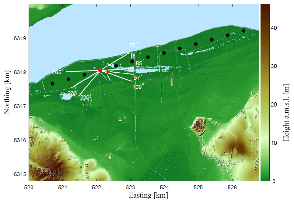
Figure 1The Nørrekær Enge wind farm in northern Denmark on a digital surface elevation model (UTM32 WGS84). The wind turbines are shown in circles, the turbine T04 with the nacelle lidars in red, and the mast as a triangle. The sectors used for the analysis are also shown; narrow direction sector: 97–109∘; wide direction sector: 97–220∘; wake sectors: 55–85 and 235–265∘. The waters of Limfjorden are shown in light blue.
2.3 Lidars
Two forward-looking lidars were installed on the nacelle of T04: a pulsed lidar (PL) with a five-beam configuration and a continuous-wave (CW) system. The CW lidar by Zephir has a single beam, which scans conically with a cone angle of 15∘ and a sampling frequency of 48.8 Hz. The CW lidar measured sequentially at five different ranges upwind from the turbine, at 0.1, 0.3, 1.0, 1.3, and 2.5 D, and it took approximately 50 s to complete a full scan at all ranges. The CW lidar measurements are binned according to the azimuthal positions in 50 bins of 7.2∘. Based on Dimitrov et al. (2019), we select 10 of these bins for further analysis and focus on ranges between 0.3 and 2.5 D, as illustrated in Fig. 2b.
The PL lidar provided by Avent technology has five fixed beams; a central beam oriented in the longitudinal direction at hub height and four beams oriented at the corner of a square pattern, as shown in Fig. 2d. The PL lidar measures simultaneously at 10 different ranges in front of the turbine 0.53, 0.77, 1.03, 1.17, 1.30, 1.53, 1.78, 2.03, 2.5, and 3.0 D, by acquiring radial velocity spectra for 1 s at each beam, thus scanning a single plane with a sampling frequency of 0.2 Hz (Peña et al., 2017). To provide a direct comparison with results from the CW lidar, we focus the analysis on the PL lidar measurements up to 2.5 D. More details of the lidars are described in Peña et al. (2017) and Dimitrov et al. (2019), while calibration reports are provided in Borraccino and Courtney (2016a, b). The top views of the PL scanning pattern and CW lidar binned data selection are illustrated in Fig. 2a, c. The lidars measure approximately within 2.5 and 5 D downstream of the wake source turbine.
We conduct the load analysis using 10 min reference periods. The dataset is filtered so that we select only periods where the turbine is operational and load, mast, and lidar measurements are available. A total of 6198 10 min periods are available in the wide direction sector, which decreases to 1042 samples in the narrow sector. The majority of measurements within the wake sectors are from westerly directions 235–265∘ with 3659 samples, while 899 samples are available from wake directions 55–85∘.
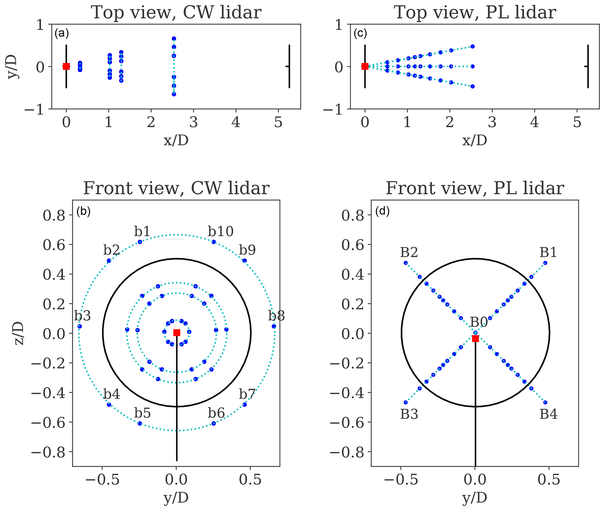
Figure 2Top and front views of the CW lidar (a, b) and PL lidar (c, d) scanning patterns shown by the blue dots. The trajectory of the lidar beams is illustrated by the dotted lines in cyan. The bins/beams notation is also given. The location of the lidars on T04 is shown with a red square marker. The reference coordinate system has an origin at the hub centre with the x axis in the mean wind direction. The distances are normalized with respect to the rotor diameter D.
Load simulations are carried out using the state-of-the-art aeroelastic HAWC2 software (Larsen and Hansen, 2007). The structural part of the code is based on a multi-body formulation assembled with linear anisotropic Timoshenko beam elements (Kim et al., 2013). The wind turbine structures (i.e. blades, shaft, tower) are represented by a number of bodies, which are defined as an assembly of Timoshenko beam elements (Larsen et al., 2013). The aerodynamic part of the code is based on the blade element momentum (BEM) theory, extended to handle dynamic inflow and dynamic stall (Hansen et al., 2004), among others.
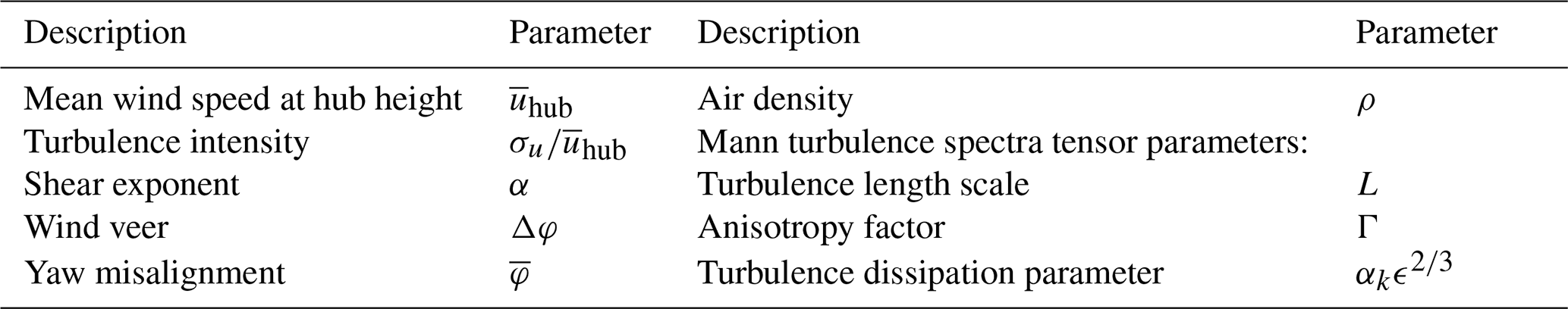
In the present study, the HAWC2 turbine model is based on the structural and aerodynamic data of the Siemens SWT 2.3-93 turbine and is equipped with the original equipment manufacturer controller. The turbulence used in the simulations is generated using the Mann turbulence model (Mann, 1994, 1998). As described in Dimitrov et al. (2018), the turbulent wind field for aeroelastic simulations can be fully characterized statistically by nine environmental parameters listed in Table 1. The methods to derive the wind field parameters from the radial velocity measurements of the nacelle-mounted lidars are described in Sect. 3.1–3.3. We propose a wake detection algorithm to detect wakes using lidar measurements in Sect. 3.4.
Table 1Wind field parameters serving as input for aeroelastic load simulations.
3.1 Wind field reconstruction
Wind field reconstruction (WFR) is defined as the process of retrieving wind field characteristics by combining measurements of the wind in multiple locations (Raach et al., 2014; Borraccino et al., 2017). As nacelle-mounted lidars measure only the line-of-sight (LOS) component of the wind vector, WFR techniques are used to derive the input wind field variables for carrying out load simulations. The present work implements the WFR technique described in Dimitrov et al. (2019). This approach assumes three-dimensional wind vectors and vertical and horizontal wind profiles combined with an induction model. The vertical wind shear is defined by a power-law profile,
where zhub is the hub height. The flow direction φ(z) is described by the combined effects of the mean yaw misalignment and the change of wind direction with height, the wind veer,
We assume a linear variation in wind direction over the rotor diameter D. To define the relation between the free-flow wind vector u=(u, v, w) and the LOS velocity uLOS, we consider a reference coordinate system with origin at hub height and co-linear with the wind turbine orientation. The wind coordinate system is aligned with the mean wind direction, which is defined by the flow direction in Eq. (2). Thus, the transformation from the wind- into the reference-coordinate system is achieved by the rotational transformation T1:
Note that the wind flow inclination (tilt) is neglected. The orientation of the LOS velocity with respect to the reference coordinate system is defined by rotations about the y and z axes, ψy and ψz (see Fig. A1). Therefore, the transformation from the LOS- into the reference-coordinate system is achieved by the rotational transformation TLOS:
As lidars measure only the LOS velocity, the first row alone of TLOS is considered. The relation between the wind vector and the LOS velocity is expressed in terms of matrix transformations as
This formulation is suitable assuming lidar point-like measurements and homogeneous wind field, which implies that the three velocity component statistics do not change over the scanned area. By combining Eqs. (1)–(5) and including an induction factor Cind based on a two-dimensional induction model (Dimitrov et al., 2019), the relation between the LOS and the wind velocity field is derived in its extended form as
The two-dimensional induction model assumes longitudinal and radial variation in the induced wind velocity. The resulting induction factor Cind is computed as
where a0 is the induction factor at the rotor centre area; is the distance from the rotor normalized by the rotor radius; is the radial distance from the rotor centre axis; and , where γa=1.1, , , λa=0.587, and ηa=1.32 (Dimitrov et al., 2019).
The parameters , α, Δφ, , a0) from Eq. (6) are to be characterized by the WFR, while x, y, and z describe the spatial location of the measurement points. The WFR approach relies on a model-fitting technique and consists in minimizing the residual between the modelled wind field and lidar measurements (Borraccino et al., 2017).
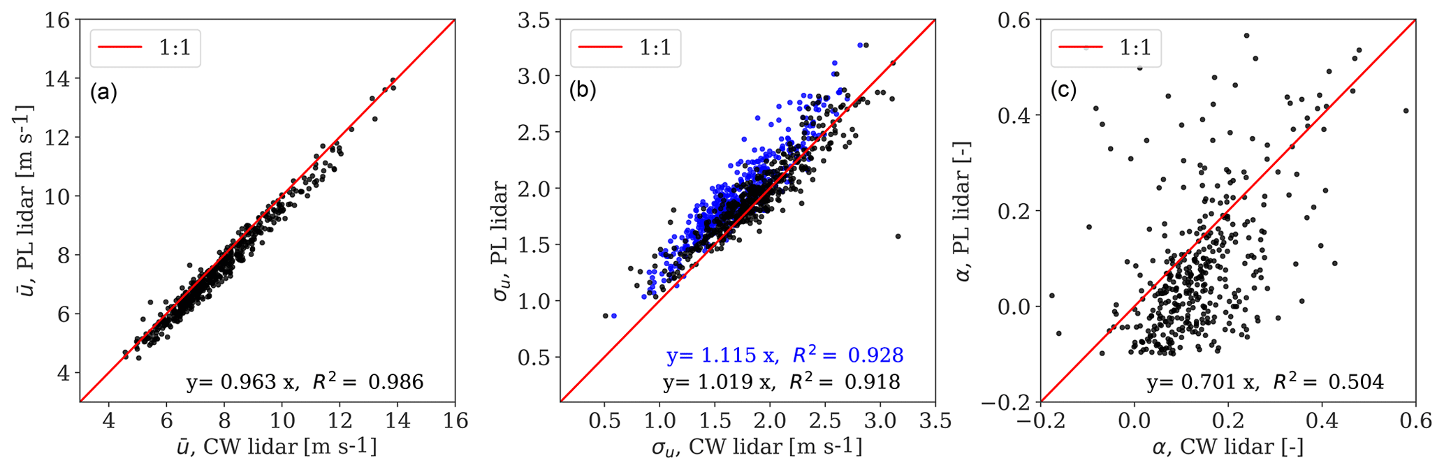
The CW and PL lidar-estimated mean wind speed in free wind, for the narrow direction sector (97–109∘), is compared with measurements from the 80 m cup anemometer mounted on the mast in Fig. 3 (left and middle). An excellent agreement is found for the lidar-estimated mean wind speed using both lidars. The lidar-estimated shear exponents are compared with the shear obtained by fitting the power-law profile using measurements from the cups at 57.5 and 80 m in Fig. 3 (right). The observed deviations result from the use of different parts of the rotor span by the PL lidar compared to the mast measurements (Dimitrov et al., 2019). In addition, the shear exponents derived by the CW lidar compare very well with those from the PL lidar (not shown).
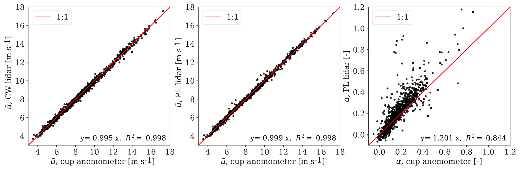
Figure 3Comparison of 10 min lidar-estimated and mast-measured inflow characteristics. We show a 1:1 line for guidance, the slope of a linear regression model and the coefficient of determination R2.
3.2 Turbulence spectral model
The wind field vector u(x) can be described by the solely spatial vector x=(x, y, z), assuming Taylor's frozen turbulence hypothesis (Mizuno and Panofsky, 1975). The statistics of velocity fluctuations (u′, v′, w′), where (′) denotes fluctuations around the mean value, are expected to be homogeneous in space (Mann, 1994). It follows that the auto- or cross-covariance function between two points can be defined only in terms of the separation distance as , where i, j=(1, 2, 3) are the indices corresponding to the components of the wind field, 〈〉 denotes ensemble averaging, and r=(r1, r2, r3) is the separation vector in the three-dimensional Cartesian coordinate system. The covariance tensor of single-point turbulent statistics () can be written as
where the matrix elements define variances and covariances of the three-dimensional velocity field u=(u, v, w). The spectral velocity tensor Φij(k) is defined as the Fourier transform of the covariance tensor,
where k=(k1, k2, k3) is the wave number vector. The spectral velocity tensor can be described by the model of Mann (1994). This model requires only three parameters: αkϵ2∕3, L, and Γ, where αk is the spectral Kolmogorov constant, ϵ is the turbulent energy dissipation rate, L is a length scale proportional to the size of turbulence eddies, and Γ is a parameter describing the anisotropy of the turbulence. Although the Mann model assumes near-neutral atmospheric conditions, the model has been applied to different surface and atmospheric stability conditions (Peña et al., 2010). The one-point spectra are computed as
The procedure to derive spectral parameters from the measured spectra of the three velocity components is described in Mann (1994). The LOS spectra measured by a lidar beam can be related to the velocity spectral tensor by accounting for probe volume effects as described in Mann et al. (2009),
where is the Fourier transform of the lidar spatial weighting function and n is the unity vector along the beam. For a CW lidar, this is typically described by a Lorentzian function (Sonneschein and Horrigan, 1971; Mann et al., 2010). For the pulsed lidar, we assume a Gaussian weighting function (Frehlich, 2013).
3.3 Turbulence characterization
Turbulence characterization using lidars is subjected to several sources of uncertainty. The measurement volumes along the LOS lead to spatial averaging of turbulence, which reduces the LOS variance when compared to a point measurement (Sjöholm et al., 2008; Sathe and Mann, 2013). Besides, the ability to properly measure the variances of the velocity components depends on the scanning strategy. Since the lidar beams are rarely aligned with any of the three velocity components, the LOS variance can be influenced by the variance of other velocity components, also referred to as cross-contamination effects.
We implement two approaches to derive filtered and unfiltered turbulence based on the work of Peña et al. (2017). The first approach uses the turbulence spectral model by Mann to correct turbulence estimates by accounting for the expected attenuation of the fluctuations of the radial velocity due to the lidar's probe volume. This can be achieved numerically by deriving the relation between the variance of the LOS velocity with and without filtering effects, respectively and . The filtering is expressed by
The magnitude of r2 varies in relation to the probe volume length Zr, turbulence characteristics, and spatial location of measurement points (Mann et al., 2010; Peña et al., 2017). Following the procedure described in Dimitrov et al. (2019), the covariance matrix of the filtered LOS velocity components RLOS can be related to the covariance of the undisturbed wind field R. To express the LOS variance as a function of the u-component variance, we normalize R with respect to . We neglect the terms and as they are small and we lack sufficient information to recover all components. Hence, we derive the ratios between variances of different velocity components using the spectral tensor model by Mann (1994),
The effects of cross-contamination and flow direction are accounted for by means of matrix transformations including TLOS and T1. The relation between the covariance matrix of the LOS components and that of the undisturbed wind field is then expressed in terms of as
where C is the induction matrix (Dimitrov et al., 2019). Note that RLOS is expressed as a full covariance matrix containing three vector components. However, as only LOS velocities are measured by the nacelle-mounted lidar, only the first component of RLOS is measured. It follows that the ratio in Eq. (14) identifies the relation between the LOS variance and the wind field variance in the longitudinal direction. As described in Dimitrov et al. (2019), the LOS residuals are calculated as the difference between the LOS measurements uLOS and the mean LOS field , α, Δφ, , a0) obtained from Eq. (6) as
Eventually, is derived by scaling the variance of the LOS residuals from Eq. (15) with the reciprocal of the filtering ratio estimated using Eq. (14). As the filtering ratio is evaluated for each LOS direction, we can combine multiple lidar measurements to estimate . The procedure is described in detail in Dimitrov et al. (2019).
The second approach avoids filtering effects by use of the ensemble-averaged Doppler radial velocity spectrum (Mann et al., 2010). This method relies on the hypothesis that the lidar average Doppler spectrum is related to the probability density function of the radial velocities (Branlard et al., 2013). This assumption is valid for homogeneous flow and for negligible velocity gradients within the probe volume. By assuming homogeneous turbulence, we use the scanning pattern to account for cross-contamination of different velocity components and extract 10 min statistics by computing the variance of Eq. (5) as
By solving the variance operator and neglecting the resulting terms and , as explained above, is derived as shown in Eq. (10) in Peña et al. (2017).
We show the comparison between lidar-estimated and mast-measured σu, using the 80 m cup anemometer, for the free-wind narrow direction sector (97–109∘) in Fig. 4. Previous work on the characterization of wind conditions at the NKE site that included wind speed and turbulence showed a discrepancy between the 76 m sonic- and 80 m cup-based mean wind speed of 2.6 % and about 12.3 % regarding the longitudinal velocity variance (Peña et al., 2017). To reduce the uncertainty of the mast-based and lidar-based wind characteristics, we choose the cup anemometer at 80 m, which is the hub height, for this analysis. The filtered turbulence derived from CW and PL lidars, using all the ranges and beams, are plotted in Fig. 4a, b, whereas the unfiltered turbulence derived from the CW lidar measurements at 1.3 D are shown in Fig. 4c. The deviations between PL lidar and the cup anemometer values are mostly due to high-frequency noise contamination as described in Peña et al. (2017). Considering the wind conditions within the free-wind narrow direction sector, the lidar-estimated turbulence compares very well with mast measurements; the observed results are consistent with previous findings (Dimitrov et al., 2019).

Figure 4(a, b) Comparison of the lidar-based σu, derived with the use of the spectral tensor model, with σu values measured with an 80 m cup anemometer mounted on the mast. (c) Comparison of lidar-based σu, derived from the ensemble-averaged Doppler spectrum of the CW lidar, with σu values measured with an 80 m cup anemometer. We show a 1:1 line for guidance, the slope of a linear regression model, and the coefficient of determination R2.
3.4 Wake detection algorithm
A wake detection algorithm is developed to determine whether the turbine is operating in free-, partial-, or full-wake situations. The algorithm relies on 10 min statistics of the lidar measurements and follows the approach of Held and Mann (2019). The idea is to detect the increase in turbulence originating from wakes with respect to the free-wind conditions. This can be done by measuring turbulence intensity TILOS and the relative turbulence difference measured by two lidar beams pointing at two opposite rotor sides, δTILOS. The detection parameters are
where B1 and B2 refer to the PL lidar beam notation given in Fig. 2. Preliminary work (Peña et al., 2017) showed that the lidar availability greatly decreases when using the bottom beams. Therefore, we use the top beams of the PL lidar for this particular analysis. Due to its location (see Fig. 1), the mast is either in the wake of T04 for wind directions coming from the south-west or in the wake of the upstream turbines for the north-east direction. As a consequence, we cannot rely on mast measurements to monitor free-wind conditions for wind directions within our range of interest. Therefore, we propose an alternative approach, which relies on lidar measurements only.
At first, we fit the wake detection parameters to a probability distribution function (pdf) using data from the wake-free wide direction sector (97–220∘). We select a log-normal and normal pdf for TILOS and δTILOS, and we choose the 99th percentile as a conservative threshold characterizing the limit of the normal range of the site-specific free-wind conditions. This results in TI and . Hence, we compare the detection parameters in wake sectors to the precomputed thresholds and classify accordingly. The parameters are shown as a function of the turbine yaw positions and classified as partial-wake (blue markers) and full-wake (red markers) in Fig. 5a, b. A partial-wake situation is detected for , whereas the sign of δTILOS indicates which half of the rotor is affected by the wake. A full wake is detected when both beams exhibit high turbulence , but . This condition appears when both beams are measuring inside the wake.
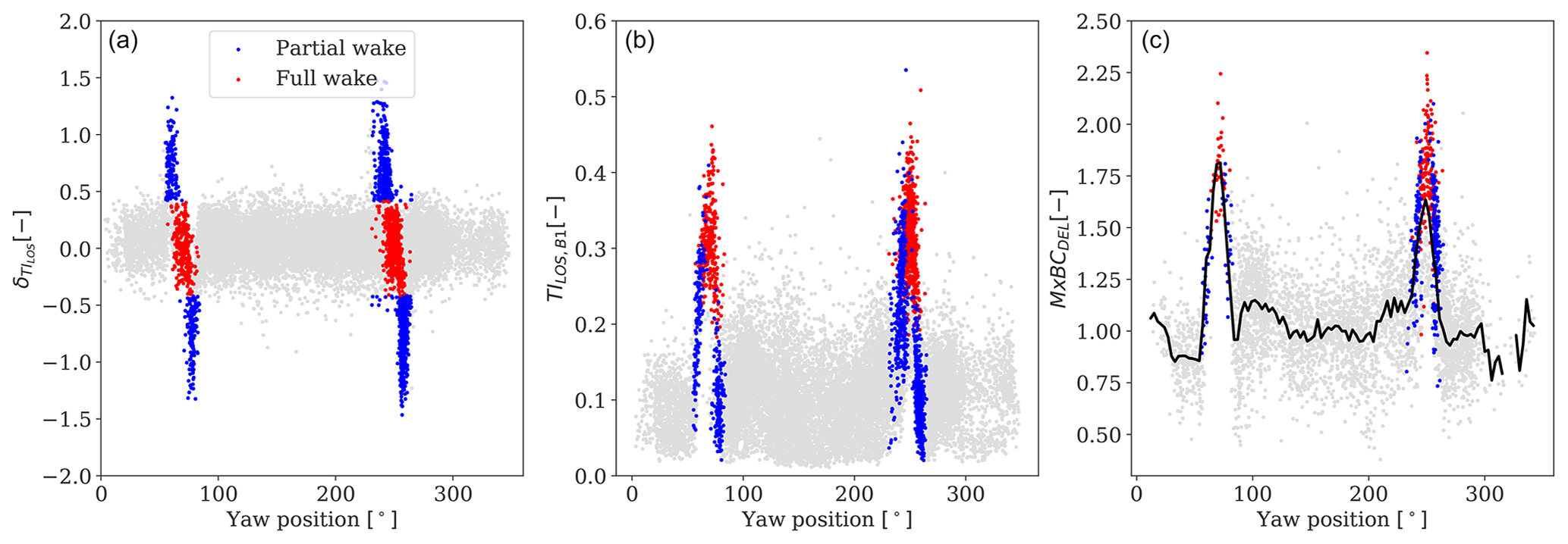
Figure 5(a, b) PL lidar-estimated 10 min wake detection parameters δTILOS and TILOS,B1, as a function of yaw position. Detected wake situations are shown with coloured markers: wake-free (grey), partial wake (blue), and full wake (red). (c) Measured blade-root flapwise fatigue loads for wind speeds between 8 and 10 m s−1, normalized over the average load levels in free-wind conditions. The black line shows the average values binned every 3∘ in direction.
Figure 5c illustrates the measured fatigue blade-root flapwise bending moments for wind speeds between 8 and 10 m s−1, as a function of the turbine orientation. Fatigue load levels are normalized with respect to the average value computed using load measurements from the free-wind wide direction sector. The 10 min periods in which the turbine is operating in wake situations are shown based on the detection algorithm. A significant wake-induced effect on the load levels can be noticed.
Further, we attempt to distinguish situations where the mast is in wake or in free wind, based on 10 min mast data. Turbulence from the cup at 80 m and shear derived from the cups at 57.5 and 80 m are used as wake detection parameters (results are shown in Fig. B1). The wake detection results presented in Fig. 5 are obtained using the PL lidar-estimated filtered turbulence at 1.3 D. An in-depth comparison between the PL and CW lidars, filtered and unfiltered turbulence estimates, and measurements at several ranges are omitted in the present work.
Improved wake detection can be obtained by establishing thresholds conditional to the ambient wind conditions (i.e. wind speed, turbulence, and atmospheric stability) and by assessing the detection parameters for shorter time periods (Held and Mann, 2019). More detailed detection algorithms including wake dynamic characteristics are proposed in the literature (Aitken and Lundquist, 2014; Aitken et al., 2014). Nevertheless, the proposed algorithm is able to detect 10 min periods where dominant wake effects are observed. The conservative thresholds ensure a strong wake influence in the inflow conditions, and a sufficient number of 10 min periods are obtained for the purpose of load validation.
The results are presented in five parts. The wake-induced effects on the reconstructed wind field parameters are analysed in Sect. 4.1 and 4.2. The wind field parameters used as input for aeroelastic simulations are derived in Sect. 4.3. The one-to-one load comparison between simulated and measured loads and their uncertainty quantification are presented in Sect. 4.4. In Sect. 4.5, we assess the sensitivity of inflow parameters on load predictions and investigate the uncertainty distribution as a function of the wind speed.
4.1 Wake effects on reconstructed wind parameters
Wind turbine wakes lead to a region characterized by reduced wind speed and increased turbulence. We observe these effects through the PL and CW lidar-estimated wind speed, turbulence, and shear exponent in Fig. 6. Here, the slope (m) of a linear regression model between the free-wind mast-measured and lidar-estimated wind parameters in free-, partial-, and full-wake situations is shown. In this particular analysis, the lidar-based wind parameters are derived from Eq. (6) evaluated at different upstream distance from the rotor without including induction effects. The 10 min periods are classified according to the results of the wake detection algorithm in Sect. 3.4, considering south-westerly directions (235–265∘). There are 287 and 175 periods respectively where partial- and full-wake situations are detected, while the mast is wake-free. The wake-free mean wind speeds range between 4 and 14 m s−1 at turbulence levels between 5 % and 15 %. Although wake effects vary according to the ambient wind field, we select all measured conditions for this comparison.
The influence of wakes on the lidar-estimated mean wind speed is shown in Fig. 6a. The reconstructed velocities in a partial wake (blue markers) and full wake (red markers) are respectively ∼5 % and ∼20 % lower than ambient wind speed. The magnitude of the velocity deficit depends on the number and location of lidar beams that are measuring inside the wake. Figure 6a also shows the influence of rotor induction at shorter ranges, where low velocity is measured in the vicinity of the turbine (Mann et al., 2018). Despite the fact that velocity recovery is expected moving downstream from the wake, the induction effects are predominant. Altogether the PL and CW lidar-estimated mean wind speeds differ from each other by less than 2 % in the analysed cases.
We compare lidar-measured σu levels inside the wake against σu measured by the mast in free wind in Fig. 6b. The bias of PL lidar-filtered turbulence (circle markers) and the CW lidar-filtered and unfiltered turbulence (star and triangle markers) are shown as a function of upfront rotor distance. The results clearly show the increased turbulence in partial and full wakes. The difference between PL and CW filtered turbulence in wake situations (circle and star markers) decreases at farther beams, where larger probe volume averaging effects are expected for the CW lidar (Dimitrov et al., 2019). The main discrepancy is found for filtered and unfiltered turbulence estimates in wake conditions, where the latter are significantly lower. We do not observe significant induction effects on the estimated σu values, as they affect the velocity variance to a much lower extent (Simley et al., 2016; Mann et al., 2018). A slight wake recovery can also be noticed, specifically in full-wake situations (red markers), where lower σu values are estimated moving downstream.
The estimated shear exponent through the PL and CW lidar for free and wake conditions is shown in Fig. 6c. As wakes expand both horizontally and vertically, wake effects can be related to a decrease in the shear exponent compared to free-wind flow and even negative values in full wakes. The differences between the PL and CW lidar-estimated shear are most pronounced in full wakes, where the CW measures at multiple points in the vertical direction. The fitted shear can also be used as an indicator of wake influence on inflow measurements.
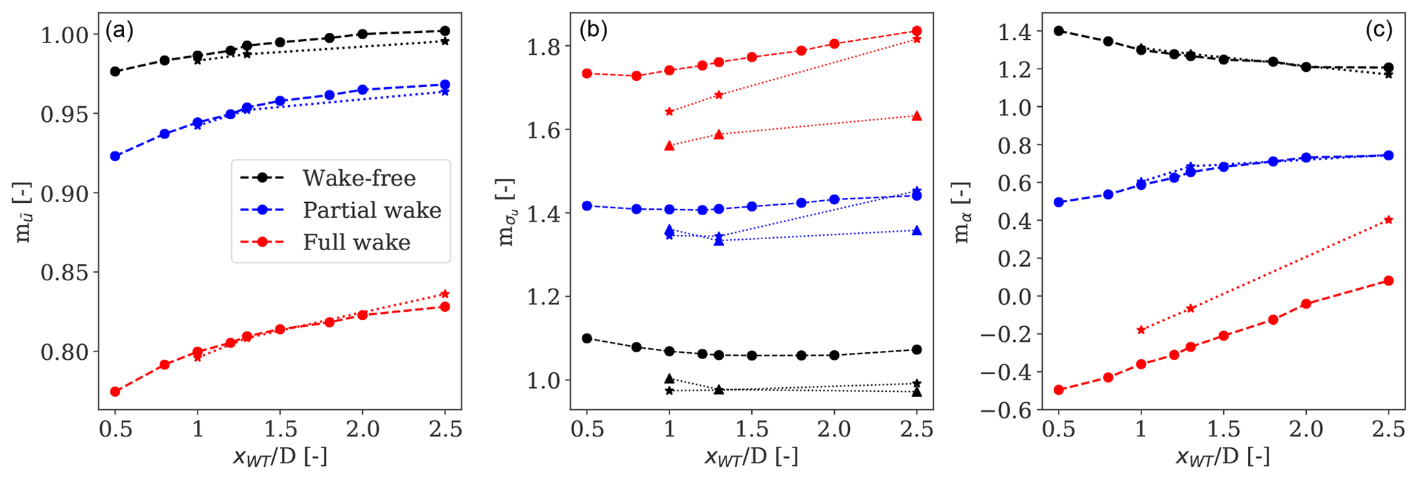
Figure 6Comparison of the slope of a linear regression model between lidar-estimated and mast-measured inflow characteristics including mean wind speed (a), the standard deviation of wind speed (b), and shear (c), when the turbine is operating in wake-free (black), partial-wake (blue), and full-wake (red) conditions and the met mast measures free-wind conditions. Results are shown as a function of lidar measuring distances in front of the rotor and normalized over rotor diameter. The results for the PL lidar are shown by the dashed line with circle markers, whereas those for the CW lidar are shown by the dotted line with star markers. The triangle markers show unfiltered turbulence obtained from the ensemble-average Doppler spectrum of the CW lidar.
4.2 Wake effects on turbulence spectral properties
In addition to the wake-induced effects on the average flow properties, turbulence spectral properties are also affected in wake regions. Earlier work on this subject showed a shift of the wake spectrum towards low length scales, compared to the free-wind spectrum, in both wind tunnel and field experiments (Vermeer et al., 2003). Although large variations in length scales occurred due to atmospheric stability, it was generally observed that wake-induced turbulence is characterized by a significantly smaller length scale than that for ambient turbulence (Chamorro et al., 2012). Furthermore, wake-added turbulence can be modelled using a synthetic turbulence field with a small length scale, as done for the DWM model (Larsen et al., 2008).
Based on these findings, we extract the turbulence spectra parameters of the Mann model, with focus on the length scale L, in free-, partial-, and full-wake situations. By comparing lidar spectra to spectra from a sonic anemometer in wake-free conditions at NKE, it was found that lidar measurements can qualitatively represent turbulence spectra, although differences increase for turbulence length scales comparable to the probe volume length (Peña et al., 2017; Dimitrov et al., 2019). We ensemble-average lidar radial velocity spectra using the central beam (B0) of the PL lidar. Assuming that the turbine is aligned with the inflow wind direction, the central beam pointing upstream at hub height is ideally measuring the wind fluctuations of the horizontal velocity component. In this case, minimal contamination effects from other velocity components are expected. Typically, three auto-spectra of the wind velocity components as well as one point cross-spectrum are fitted simultaneously to the theoretical spectra to derive the Mann model parameters. However, as we measure a single LOS spectrum, we assume Γ=3, which is suitable for the terrain and climate for free-wake conditions (Peña et al., 2017). Although Γ impacts load predictions, the influence of the turbulence length scale was found to be predominant (Dimitrov et al., 2017, 2018).
The 10 min time series of radial velocity are classified into free-, partial-, and full-wake situations and the spectra are ensemble-averaged over all conditions within each class. Then, the parameter L is fitted to the ensemble-averaged spectrum. The comparison is based on the energy spectra of the u-velocity component (along-wind) in free-, partial-, and full-wake situations. The measured and theoretical spectra, normalized over the relative variance, are shown in Fig. 7a. The aggregated measured spectra in wakes show a shift of spectrum peak towards higher wave numbers, as expected, which indicates high energy content at low turbulence length scales. The deviations between the modelled and the measured spectra increase under wake situations. This follows from the limitations of the Mann model, which was developed for homogeneous wind flow and near-neutral atmospheric conditions; the constraints of the adopted fitting procedure; and the uncertainty of the lidar-measured spectra. In fact, the derived length scale values are critically affected by the probe volume filtering effects, atmospheric stability conditions, sampling frequency, and measurement location in the wake region. Resulting length scales of approximately 35, 15, and 7 m are estimated, respectively, for free-, partial-, and full-wake conditions. These values are used to generate synthetic turbulence fields for load simulations.
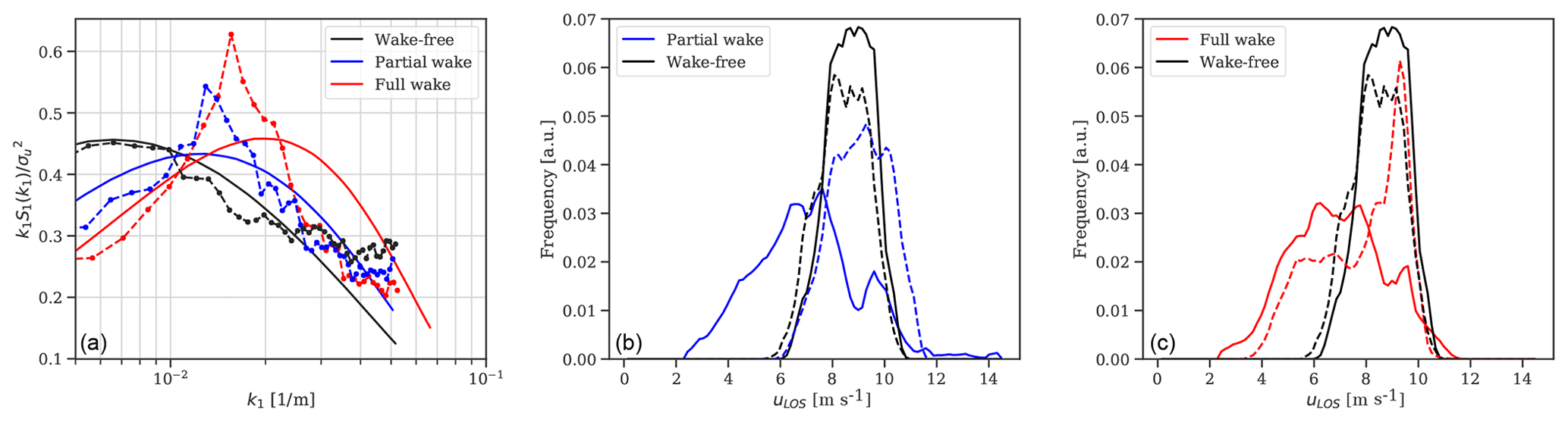
Figure 7(a) Comparison of the normalized ensemble-average uLOS spectrum based on measurements with the central beam of the PL lidar (dashed line and markers) against the fitted theoretical Mann spectra using Eq. (11) (solid line). (b, c) Normalized ensemble-average Doppler spectrum measured over a 10 min period by the CW lidar using bins b3 (solid line) and b8 (dash line).
The small-scale turbulence generated within wake flows generally leads to a significantly larger broadening of the Doppler spectrum compared to that in the ambient flow (Branlard et al., 2013; Held and Mann, 2019). We show an example of a 10 min ensemble-average Doppler spectrum obtained from the radial velocity of the CW lidar using bins b3 and b8 (see Fig. 2 for notation) at 1.3 D in partial-wake and full-wake conditions in Fig. 7b, c. We also provide the ensemble-average Doppler spectrum in free wind for reference. For this comparison, we select three 10 min periods with similar inflow conditions measured at the mast; thus m s−1 and . It can be noticed that broadening effects are present only in b3 (solid blue line) in the partial-wake situation and in both bins (solid and dashed red lines) in full-wake conditions.
4.3 Reconstructed inflow parameters for load simulations in wake situations
We select around 500 10 min samples for each of the free-, partial-, and full-wake scenarios, which are distributed within the wind speed range 4–14 m s−1. We select 10 min periods within the narrow sector (97–109∘) for free-flow conditions and periods of south-west directions (235–265∘) for wake situations. The main limitation of the current dataset is given by the concurrent availability of both lidars and by the few 10 min periods at high wind speeds in full-wake situations.
The comparison of the reconstructed wind field characteristics in partial-wake conditions using PL and CW lidar measurements from all ranges is presented in Fig. 8. A very good agreement can be observed for the mean wind speed; the line fits yield slopes of nearly unity and an R2 of almost 100 %. The filtered turbulence from the PL lidar is ∼2 % lower than that from the CW lidar. The differences can be partly explained by the larger amount of filtering occurring for farther beams of the CW lidar as well as due to the distinct scanning patterns measuring an inhomogeneous wind flow. When compared to the filtered turbulence, the unfiltered estimations show a significant reduction by ∼6 % (blue markers in Fig. 8b). A large scatter appears for the shear, veer, and yaw (the latter two are not shown), which are subjected to a high level of uncertainty and highly depend on the scanning patterns. Similar results are found for the full-wake situation as presented in Fig. 9. The main discrepancy is in the estimation of the shear exponent.
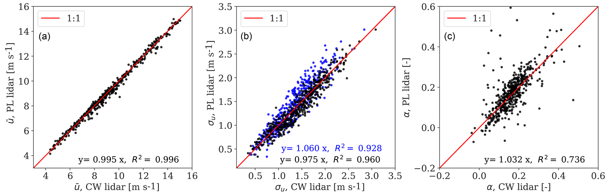
Figure 8Comparison of the CW and PL lidar 10 min reconstructed wind speed (a), filtered and unfiltered turbulence in black and blue colour, respectively (b), and shear exponent (c) for partial-wake conditions. We show a 1:1 line for guidance, the slope of a linear regression model, and the coefficient of determination R2.
4.4 Load validation procedure
The load validation analysis is conducted on the dataset described in Sect. 4.3. We analyse about 500 10 min samples distributed between 4 and 14 m s−1, for free-, partial-, and full-wake scenarios. The quality of load predictions is evaluated through one-to-one comparisons against load measurements. The resulting statistics from HAWC2 simulations are denoted by () and the corresponding measured statistics from the turbine on-board sensors by (). Three uncertainty-related indicators are assessed, where the symbol E(.) denotes the mean value and 〈.〉 the ensemble average.
-
coefficient of determination ;
-
uncertainty ;
-
bias .
The R2, XR, and ΔR indicators are computed for free-, partial-, and full-wake situations. The 10 min wind turbine statistics investigated hereafter include the mean power production (Powermean), the extreme loads, and 1 Hz damage-equivalent fatigue loads of fore–aft tower bottom bending moment (, ) and flapwise bending moment at the blade root (, ). Note that given the strain gauge convention, the increasing flapwise bending moment results in negative loading; thus we refer to as the extreme loads (Dimitrov et al., 2019). Therefore, time series of 600 s are simulated in the aeroelastic code HAWC2, and load statistics are derived at the location where the strain gauges are installed. A turbulence seed with statistical properties matching those of the measured 10 min conditions is input to the load simulations.
The rain flow counting algorithm is used to compute the 1 Hz damage-equivalent fatigue loads with a Wöhler exponent of m=12 for blades and m=4 for the tower. The same approach is used to post-process measured loads. We run simulations using wind field characteristics listed in Table 1, which are derived from both the PL and CW lidars as well as the mast measurements. A more detailed analysis is conducted for partial- and full-wake situations. Here, we investigate how power and load predictions are influenced by filtered and unfiltered turbulence estimates derived in Sect. 4.3, characteristic turbulence length scales derived in Sect. 4.2, and wind parameters derived from lidar measurements at several ranges.
We provide detailed scatter plots of measured and predicted load sensors used in the analysis in Figs. C1–C5. The prediction uncertainties for power production and extreme loads are presented in Table 2 and for fatigue loads in Table 3. We define the lidar-based power and load predictions in free wind as the reference case. Thus, we compare the relative error between the uncertainty indicators derived from wake situations with that from the free-wind case. Generally, we observe lower prediction accuracy in partial- and full-wake situations compared to the free-wind scenario, while in some cases similar uncertainty levels are obtained. The following sections describe the results in detail.
Table 2List of accuracy and uncertainty values for power and extreme load validation procedures. The marker indicates unfiltered turbulence obtained from the ensemble-average Doppler spectrum of the radial velocity at 1.3 D.

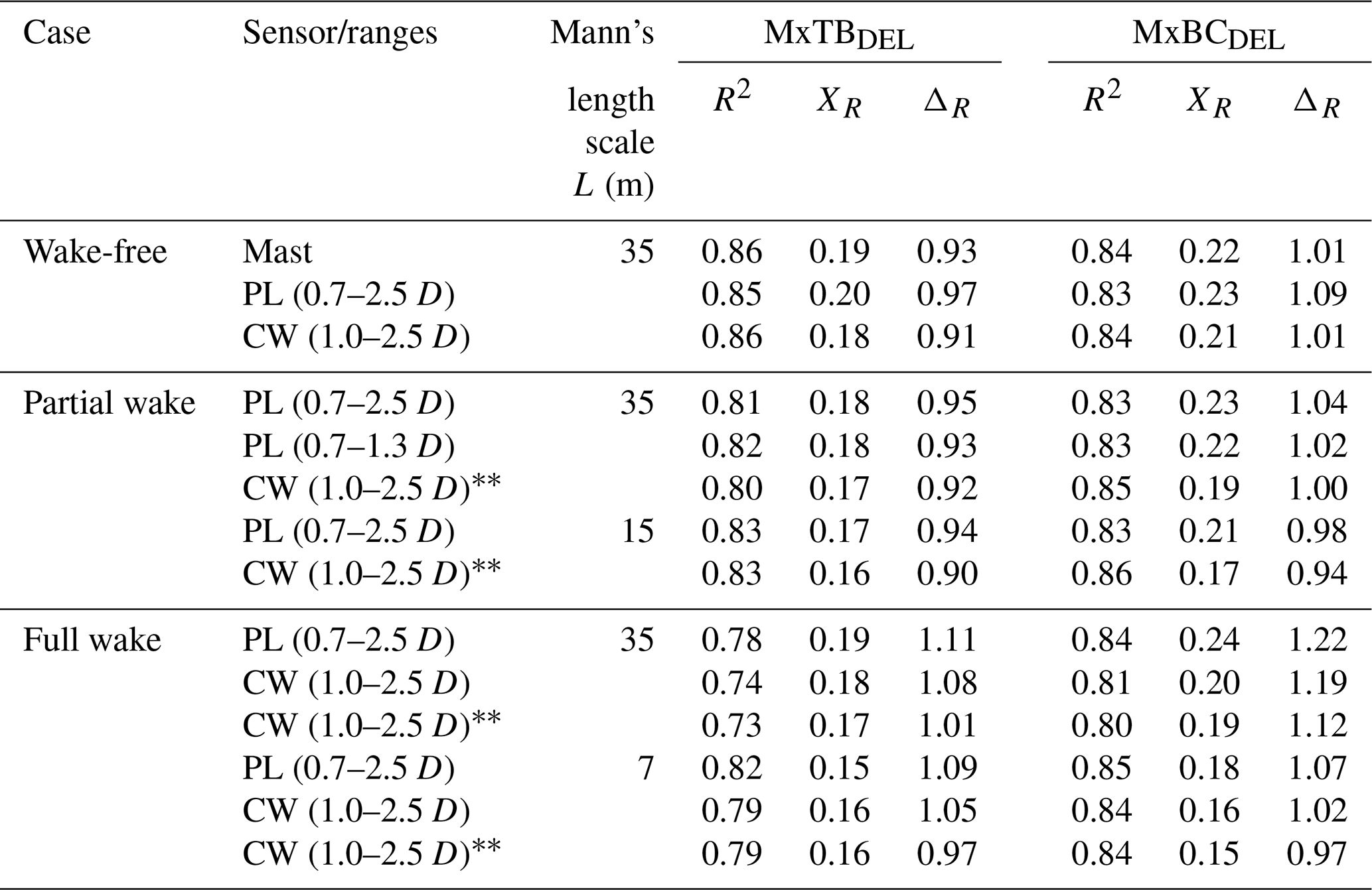
Table 3List of accuracy and uncertainty values for fatigue load validation procedures. The marker indicates unfiltered turbulence obtained from the ensemble-average Doppler spectrum of the radial velocity at 1.3 D.
4.4.1 Power predictions
Power production levels are overestimated in the partial wake but underestimated in the full wake by approximately 4 % compared to the free-wind case. Larger XR values are found in the full wake compared to the reference case, although R2 is above 96 %, which indicates a good correlation. We do not observe a significant influence of turbulence intensity levels on power predictions, i.e. by comparing the uncertainties in the full wake between simulations performed with filtered and unfiltered turbulence estimates from the CW lidar in Table 2. In a similar way, small turbulence length scales derived in wakes have a negligible effect on power production levels. The power prediction deviations in the partial wake drop to approximately 1 %, when the PL lidar-estimated wind characteristics using measurements up to 1.3 D are used in the simulations. This result indicates the sensitivity of the reconstructed wind field characteristics to the upstream ranges in a strongly inhomogeneous wind field as a partial-wake situation.
4.4.2 Extreme load predictions
The extreme loads (, ) are affected by both the turbulence levels and the turbulence length scale. We obtain similar deviations in partial- and full-wake conditions to the free-wind conditions, when using unfiltered turbulence estimates and length scales extracted in free-wind conditions (see Table 2). However, simulations based on filtered turbulence consistently overestimate extreme load levels (3 %–7 %). The effect of a low value for the length scale is noticeable in full-wake situations, where L=7 m leads to biases of the order of −7 % compared to the reference case. Overall, higher XR values are derived in wakes compared to the reference, while R2 remains above 89 % in all analysed cases. It should also be noticed that the maximum loads do not increase significantly in wake situations, since the wind speed in the wakes is lower than the free wind (Larsen et al., 2013).
4.4.3 Fatigue load predictions
The biases of fatigue load predictions in the partial wake, using unfiltered turbulence statistics and L=35 m, are comparable with the deviations observed in free-wind conditions, as seen in Table 3. The error increases when filtered turbulence from the PL lidar is used for the simulations, leading to an underestimation of fatigue loads between 2 % and 5 %. The most significant deviations are observed for and in full-wake conditions. The simulations based on filtered turbulence measures and L=35 m lead to an overestimation of blade-root and tower-bottom predictions by 21 % compared to the free-wind case. The filtered turbulence statistics are predicted with the use of the spectral velocity tensor model and are found to be approximately 11 % higher compared to unfiltered turbulence derived from the Doppler radial velocity spectrum (see Fig. 9b). The bias of fatigue load predictions drops to approximately 11 %, when unfiltered turbulence measures from the CW lidar are simulated. Overall, extreme and fatigue load predictions show low uncertainty when unfiltered turbulence estimates are used as input in simulations.
Fatigue loads are found to correlate significantly better when a synthetic turbulent field characterized by small length scales is used (i.e. L=7 m). This is demonstrated by improved XR and R2 indicators compared to those resulting from simulations with L=35 m. Besides, reducing L from 35 m (free-wind conditions) to 7 m (fitted in full-wake conditions) reduces fatigue blade-root load levels by 15 %. The simulations with low length scales and unfiltered turbulence measures provide the lowest deviations in full-wake conditions compared to the reference case, as the error drops to −4 % for , indicating underprediction (see Table 3). These results demonstrate the improved accuracy of load predictions when unfiltered turbulence measures are simulated and validate the importance of characterizing turbulence spectral parameters for load analysis, as previously demonstrated in Thomsen and Sørensen (1998), Sathe et al. (2012), and Dimitrov et al. (2017).
4.5 Sensitivity of inflow parameters on load predictions
We use a first-order polynomial response surface for evaluating the sensitivity of the predictions with respect to input wind variables. We consider , , α, Δφ, , and L in the analysis. The first-order polynomials are separately fitted for free-, partial-, and full-wake conditions based on the PL lidar-measured wind field parameters. We ensure close to 850 10 min samples for each case. Besides, L is assumed to randomly vary between 7 and 30 m in full-wake conditions and between 15 and 35 m in partial-wake and free-wake situations. We normalize the input variables such that their values are scaled between zero and 1 to allow the sensitivity study.
The obtained linear regression coefficients for Powermean, , and responses are presented in Fig. 10. Similar trends are obtained for and (not shown). The power predictions are strongly driven by the reconstructed mean wind speed at hub height as shown in Fig. 10a. This indicates that the observed ΔR values in Table 2 are mostly explained by the uncertainty in the wind speed reconstruction. The mean wind speed and turbulence intensity have the largest influence on the fatigue load predictions (see Fig. 10b). In comparison to the wake-free scenario, we observe the increased effect of turbulence intensity and reduced influence of shear exponents in wake situations. This is due to the significantly high turbulence levels measured inside the wakes (up to 1.8 times higher than under free-wind conditions) and relatively low shear exponent values (see Fig. 6). The former is a well-known fatigue load driver. The latter implies small velocity gradients within the rotor area, which lead to lower blade-root fatigue loads (Sathe et al., 2012; Dimitrov et al., 2015). The effects of α, Δφ, , and L are secondary compared to and . We observe slightly higher sensitivity of L in full-wake conditions compared to partial-wake and free-wind conditions. However, according to the results in Table 3, the length scale parameter has a significant impact on loads when assessed independently. Finally, and have the largest influence on the extreme tower bottom loads in Fig. 10c. Overall, the order of importance of the analysed inflow parameters are comparable with the more detailed sensitivity studies provided in Dimitrov et al. (2018).
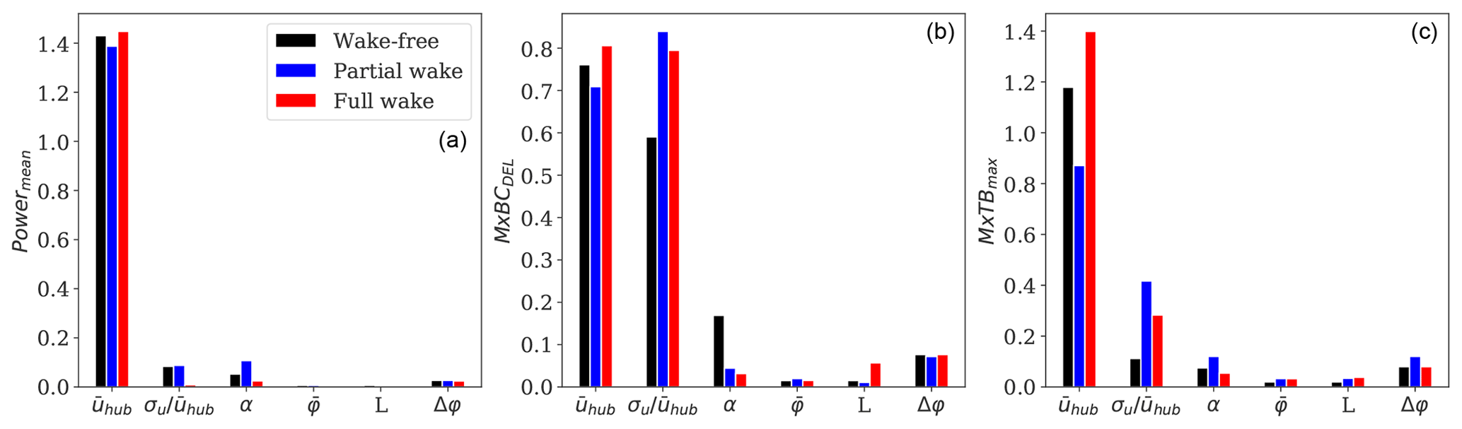
Figure 10Regression coefficients of a linear response surface model identifying the sensitivity of wind field parameters to (a) mean power production, (b) fatigue flapwise bending moment at the blade root, and (c) extreme fore–aft tower bottom bending moment.
4.5.1 Uncertainty distribution as a function of wind speed
We analyse the bias and uncertainty of Powermean, , and predictions with respect to the inflow wind speed in Fig. 11. We observe larger deviations of the selected sensors at low wind speeds, which gradually decrease for higher winds. The deviations in the reference case (black line) and wake situations are a combination of uncertainty in the reconstructed wind profiles, aeroelastic model uncertainty, load measurement uncertainty, and statistical uncertainty (Dimitrov et al., 2019). Although there is not sufficient information to distinguish among the various uncertainty sources, we assume that the deviations are due to the error in the wind field representation only.
The power prediction uncertainties with respect to mean wind speed in free-, partial-, and full-wake situations are plotted in Fig. 11a. We observe a consistent overprediction of power levels in partial-wake conditions (blue line) and underprediction in full-wake conditions (red line) for the full range of wind speeds. The predictions of with respect to the mean wind speeds in free- and full-wake conditions are plotted in Fig. 11b. The predictions based on the unfiltered turbulence (green line) show better agreement with the reference compared to results based on filtered turbulence (red line). It is also found that the largest deviations occur at low wind speeds ( m s−1). Finally, we show the results using unfiltered turbulence and a low length scale (purple line), which provide the lowest error. The residual deviations can be partly explained by the uncertainty in turbulence statistics and spectral property representation. Figure 11c shows that comparable deviations are obtained for tower extreme loads in partial- and full-wake situations as for the reference case.
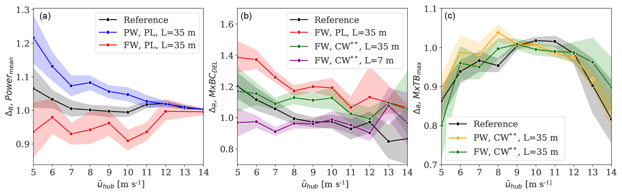
Figure 11Comparison of bias (solid line) and uncertainty (error band) of (a) mean power production, (b) fatigue flapwise bending moment at the blade root, and (c) extreme fore–aft tower bottom bending moment, with respect to inflow mean wind speed. The analysed cases are shown with coloured lines in each sub-plot. The reference case denotes the mast-based free-wind scenario; PW refers to partial-wake conditions and FW refers to full-wake conditions. We show results from both PL and CW lidars and different turbulence length scales L. The marker indicates unfiltered turbulence obtained from the ensemble-average Doppler spectrum of the radial velocity at 1.3 D.
Wind field parameters used as inputs for aeroelastic simulations are derived from PL and CW lidar measurements of the wake field behind an operating wind turbine. Although the two lidars follow different scanning patterns and the wake flow field is strongly inhomogeneous, we find a very good agreement between the PL and CW lidar-estimated horizontal wind speed and filtered turbulence in partial- and full-wake situations. The estimation of the wind veer, yaw error, and shear exponent using nacelle-mounted lidars is prone to a high level of uncertainty and is affected by the scanning patterns. This is demonstrated by the larger scatter between the estimated parameters by the PL and CW lidars in wake compared to free-wind conditions (not shown). However, we demonstrate that the influence of these parameters on the loads and power predictions is minor compared to mean wind speed, turbulence intensity, and length scale.
Although the present work does not focus on details of the performance of the two lidar systems, the findings indicate that the main sources of uncertainty in load predictions are related to flow modelling assumptions. The wind velocity gradient in the wake is characterized by the combined effect of the atmospheric shear and the wake deficit. The former can be explained by a power-law profile, while the latter is often approximated in the far wake by a bivariate Gaussian shape function, whose depth and width depend on ambient conditions and turbine operation regimes (Trujillo et al., 2011; Aitken et al., 2014). Further, the 10 min average wind velocity gradient, observed from a fixed point, will be largely influenced by wake meandering in the lateral and vertical directions, increasing the complexity of the velocity field in the wake region. The results of the power prediction's deviations in Table 2, in both partial- and full-wake situations, indicate a less accurate reconstruction of the wind field when compared to wake-free conditions. Although we demonstrate a low sensitivity of the loads to the shear exponent for all the analysed sensors (see Fig. 10), it is envisioned to more appropriately account for wake-affected velocity gradient profiles, which include a wake shape function and the contribution of the meandering, and determine whether or not this will significantly improve the accuracy of power and load predictions.
It is well-established that fatigue loads are dominated by turbulence levels. However, to extract turbulence parameters by combining a turbulence model with a model of the spatial radial velocity, averaging of the lidars introduces significant uncertainty under wake conditions. Indeed, filtered turbulence estimates in wakes are 6 %–10 % higher than unfiltered turbulence measures, derived from the Doppler radial velocity spectrum, as shown in Figs. 8 and 9. We describe the wake flow as a homogeneous field by using the Mann spectral tensor model fitted using PL lidar measurements at hub height. Nonetheless, wake fields are highly inhomogeneous, and spectral properties vary significantly within the rotor region (Kumer et al., 2017). We derive turbulence length scales in wakes and demonstrate the importance of characterizing turbulence spectra for the load analysis. The observed magnitude of decrease in longitudinal turbulence length scale is consistent with results reported in Thomsen and Sørensen (1998) and Madsen et al. (2010), where wake-added turbulence is characterized by length scales within the range 10 %–25 % of the free-wind length scale. However, a detailed analysis including atmospheric stability effects on both turbulence spectra and wake characteristics can potentially reduce the uncertainty of load predictions (Sathe et al., 2012; Dimitrov et al., 2017). Furthermore, cross-contamination effects and probe volume averaging effects become larger in wakes, as the size of turbulence eddies decreases to length scales comparable to or lower than the lidar probe volume. These effects increase the uncertainty of extracted turbulence length scales from lidar measurements. Despite this, fatigue load predictions show significant improvement by using low turbulent length scales; spectral analysis of measured and predicted loads is required for a better understanding of the accuracy of the lidar-fitted synthetic turbulence field in wakes.
We demonstrate that improved fatigue load predictions are obtained using unfiltered turbulence measures from the Doppler radial velocity spectrum. However, the estimation of from the relies on flow homogeneity and Taylor's frozen turbulence hypothesis (Taylor, 1938). These assumptions are sound for large-scale wind fluctuations and free flow over flat and homogeneous terrain but not valid in wakes (Schlipf et al., 2010). The current wind field modelling approach omits the large-scale meandering of wakes, which has a strong impact on power and load predictions (Larsen et al., 2013). These uncertainty sources, among others, can partially explain the observed deviations.
The influence of wake effects on power and load levels depends on the wind farm layout, ambient wind speed and turbulence, and atmospheric stratification, among others. The current state-of-the-art approach to predict wake flows and their influence on wind turbine operations relies on engineering-like wake models (Frandsen, 2007; Madsen et al., 2010). These models ensure an acceptable level of accuracy, robustness, and computational cost. Previous studies carried out load validation using the effective turbulence model and the DWM model, which are recommended in IEC 61400-1. As described in Sect. 1, results from these studies show deviations of the same or even larger order of magnitude compared to the results from our load validation approach. Despite the discussed shortcomings, load validation under wake conditions based on lidar measurements may already be a viable alternative to the engineering wake models. We will soon evaluate whether the differences in the calculated loads using lidar-estimated wind characteristics in wakes are larger compared to the uncertainties in the load calculations with state-of-the-art wake models such as DWM.
We demonstrated a procedure for carrying out load validation in partial- and full-wake conditions using measurements from two types of forward-looking nacelle lidars: a pulsed- and continuous-wave system. The suggested procedure characterized wake-induced effects by means of lidar-reconstructed wind field parameters commonly used as input for load simulations, without applying wake deficit models.
We considered the uncertainty of lidar-based load predictions against wind turbine on-board sensors in free-wind conditions as the reference case. Hence, we quantified the uncertainty of lidar-based load predictions against sensor data in wake conditions, and we compared it to uncertainty of the free-wind case. The reconstructed mean wind speed, turbulence intensity, and turbulence length scale in wake conditions were found to be the most influential parameters on the predictions.
Power production levels under wake conditions were strongly driven by the reconstructed wind speed at hub height, whereas turbulence intensity as well as turbulence length scales had negligible effects on those levels. Power predictions were overestimated in partial-wake conditions but underestimated in full-wake conditions by approximately 4 % compared to on-board sensors, while free-wind conditions were unbiased.
Fatigue loads were affected by turbulence characteristics inside the wake. The use of a spectral velocity tensor model to derive turbulence parameters introduced significant uncertainty under wake conditions. The tower-bottom and blade-root bending moment predictions were overestimated by 21 % in full-wake conditions using filtered turbulence measures and turbulence length scales typical of free-wind conditions. The bias was reduced to 11 % using unfiltered turbulence measures derived from the ensemble-average Doppler radial velocity spectrum.
Overall, the measured and predicted fatigue and extreme loads were found to correlate significantly better when a synthetic turbulent field characterized by a low turbulence length scale was used. Furthermore, simulations with low turbulence length scales led to an underestimation of blade-root fatigue load predictions by 4 % compared to on-board sensors, while free-wind situations were unbiased. However, estimating turbulence characteristics under wake conditions using measurements from nacelle-mounted lidars was prone to a high level of uncertainty due to probe volume effects and flow modelling assumptions.
The present work demonstrated the applicability of nacelle-mounted lidar measurements to extend load and power validations under wake conditions and highlighted the main challenges. Further investigation is necessary to verify that the observed uncertainty of predictions is comparable with results using state-of-the-art wake models recommended by the IEC standard. Future research should apply a wind deficit model that accounts for the combined effect of atmospheric shear and wake deficit and quantify the uncertainty of resulting power and load predictions.

Figure A1Schematic view of the measurement patterns of nacelle-mounted lidars: CW lidar (a) and PL lidar (b).
The wake detection algorithm (see Sect. 3.4) is extended to the mast measurements to classify 10 min periods where the mast is in free or wake situations. For this purpose, turbulence observations from the cup anemometer at 80 m and vertical wind shear computed using the measurements from the cup anemometers at 57.5 and 80 m are used as wake detection parameters. Their 99th percentiles are used as conservative thresholds to characterize the limits of the normal range of the site-specific free-wind conditions. The resulting thresholds are TI and . If one of the two limits is exceeded within a 10 min period, the mast is considered in wake conditions and shown with green markers in Fig. B1.
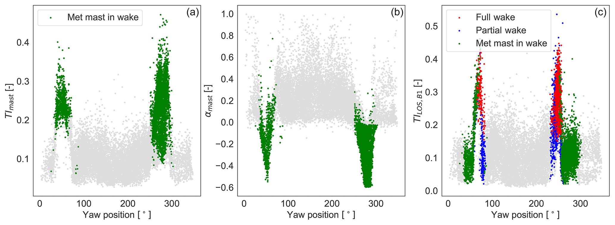
Figure B1(a, b) The 10 min observations of the turbulence intensity and vertical wind shear at the mast as a function of turbine yaw position. Free-wind conditions relative to the mast are identified with grey markers, and waked situations are identified with green markers. (c) PL-estimated 10 min wake detection parameter TILOS,B1. Detected wake situations of turbine T04 are shown with coloured markers: wake-free (grey), partial-wake (blue), and full-wake (red) conditions. The 10 min periods when the mast is affected by wakes are shown as green markers.

Figure C1Scatter plots of the normalized measured and predicted power mean realizations used in the analysis.
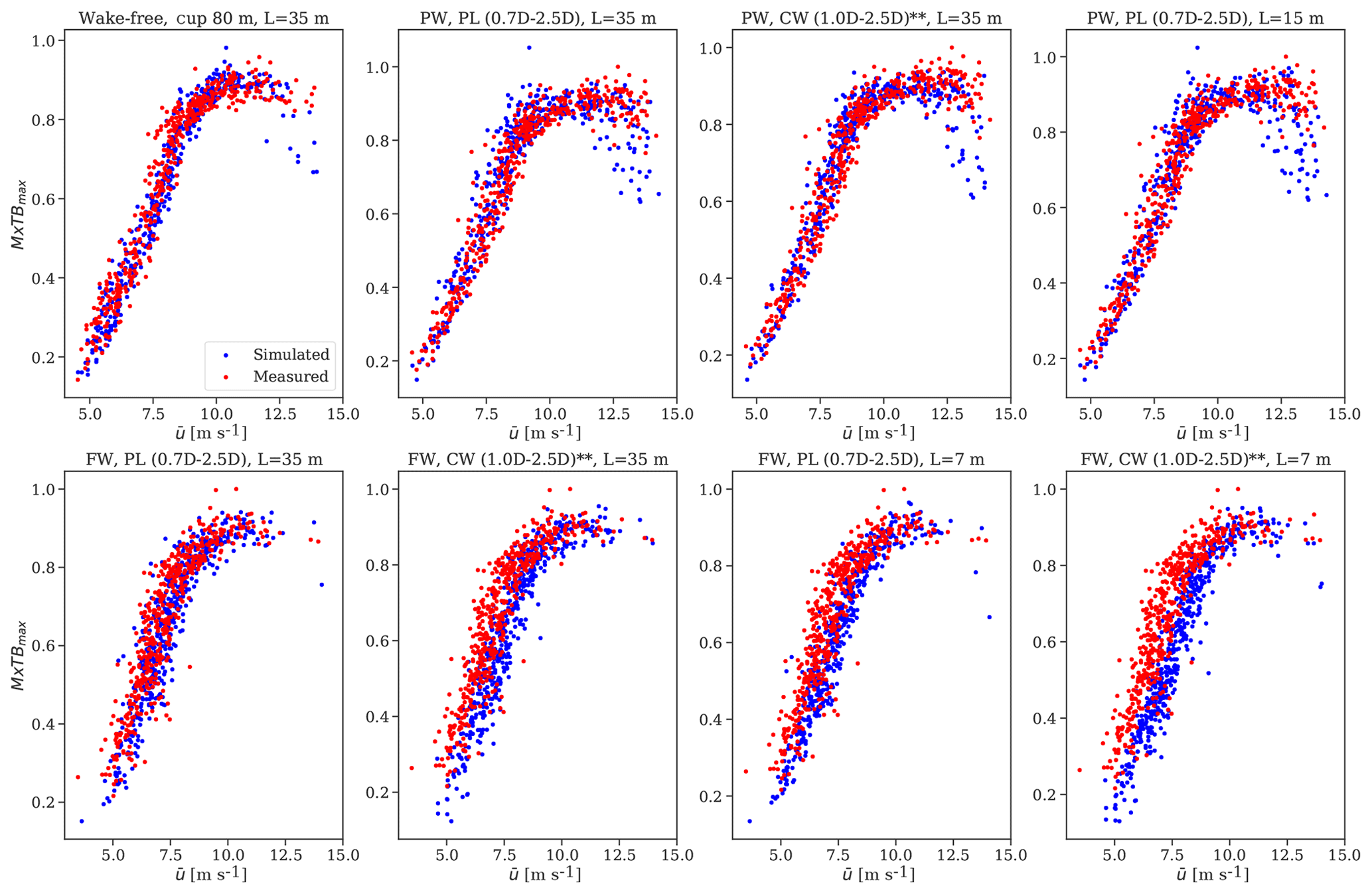
Figure C2Scatter plots of the normalized measured and predicted extreme fore–aft tower bottom bending moment realizations used in the analysis.
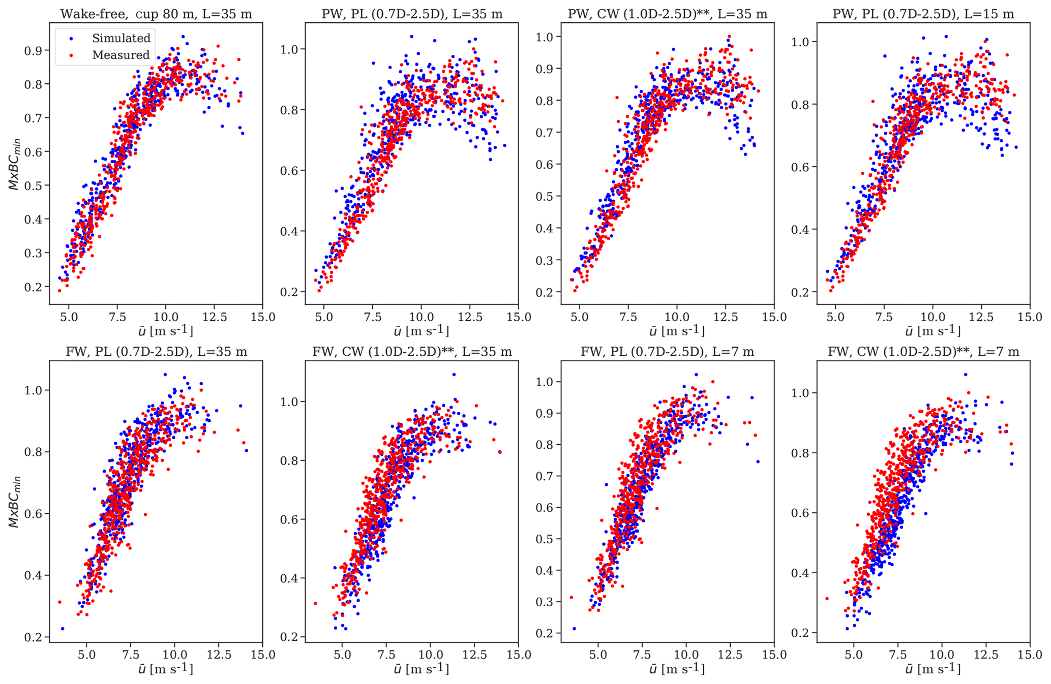
Figure C3Scatter plots of the normalized measured and predicted extreme flapwise bending moment at the blade-root realizations used in the analysis.
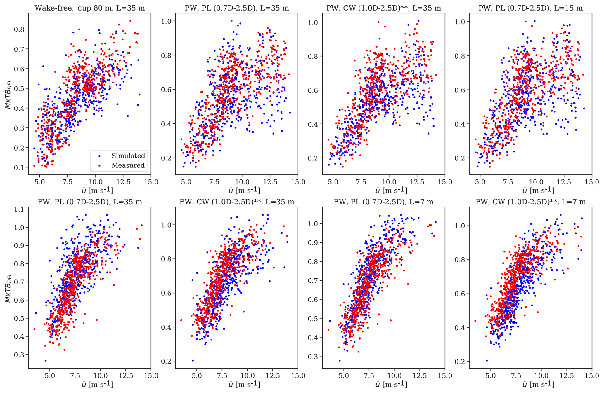
Figure C4Scatter plots of the normalized measured and predicted fatigue fore–aft tower bottom bending moment realizations used in the analysis.
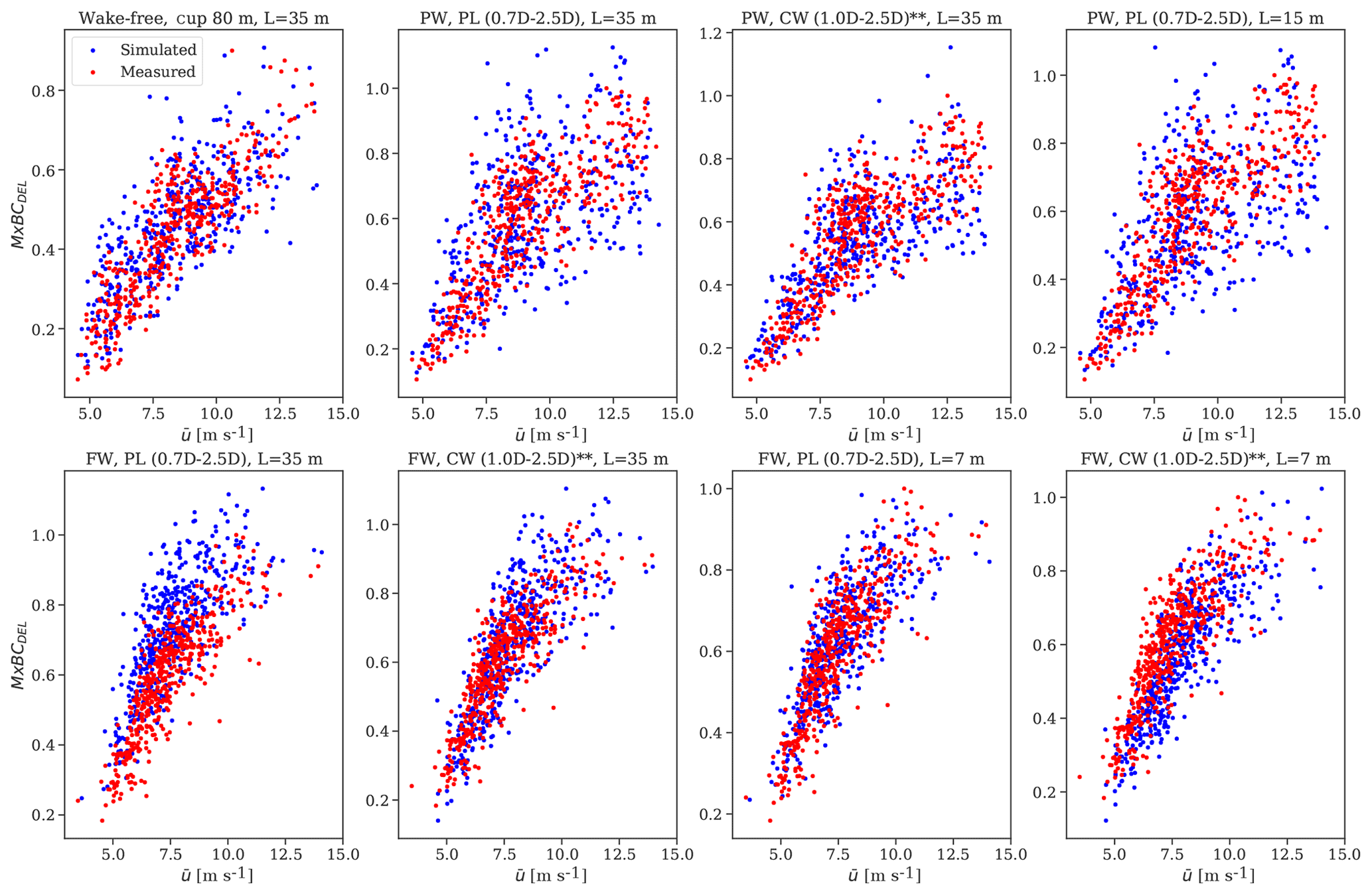
Figure C5Scatter plots of the normalized measured and predicted fatigue flapwise bending moment at the blade-root realizations used in the analysis.
Turbine data are not publicly available because there is a non-disclosure agreement between the partners in the UniTTe project. Lidar and mast data can be requested from Rozenn Wagner at DTU Wind Energy (rozn@dtu.dk).
DC, ND, and AP participated in the conception and design of the work. DC conducted the data analysis, carried out aeroelastic simulations, and wrote the draft manuscript. ND and AP contributed with the acquisition of the dataset, provided key elements of the programming code, supported the overall analysis, and critically revised the manuscript.
The authors declare that they have no conflict of interest.
This article is part of the special issue “Wind Energy Science Conference 2019”. It is a result of the Wind Energy Science Conference 2019, Cork, Ireland, 17–20 June 2019.
Special thanks to Rozenn Wagner for making the NKE dataset available for our study. Thanks to the lidar manufacturers from Avent and Zephir for providing their systems. Thanks to Vattenfall and Siemens Gamesa Renewable Energy for providing the site and turbine to conduct the measurement campaign.
This paper was edited by Julie Lundquist and reviewed by two anonymous referees.
Aitken, M. L. and Lundquist, J. K.: Utility-scale wind turbine wake characterization using nacelle-based long-range scanning lidar, J. Atmos. Ocean. Tech., 31, 1529–1539, https://doi.org/10.1175/JTECH-D-13-00218.1, 2014. a
Aitken, M. L., Banta, R. M., Pichugina, Y. L., and Lundquist, J. K.: Quantifying wind turbine wake characteristics from scanning remote sensor data, J. Atmos. Ocean. Tech., 31, 765–787, https://doi.org/10.1175/jtech-d-13-00104.1, 2014. a, b
Bingöl, F., Mann, J., and Larsen, G. C.: Light detection and ranging measurements of wake dynamics Part I: One-dimensional Scanning, Wind Energy, 13, 51–61, https://doi.org/10.1002/we.352, 2010. a
Borraccino, A. and Courtney, M.: Calibration report for ZephIR Dual Mode lidar (unit 351), Technical Report DTU Wind Energy E-0088, DTU Wind Energy, Roskilde, Denmark, 2016a. a
Borraccino, A. and Courtney, M.: Calibration report for Avent 5-beam Demonstrator lidar, Technical Report DTU Wind Energy E-0087, DTU Wind Energy, Roskilde, Denmark, 2016b. a
Borraccino, A., Schlipf, D., Haizmann, F., and Wagner, R.: Wind field reconstruction from nacelle-mounted lidar short-range measurements, Wind Energ. Sci., 2, 269–283, https://doi.org/10.5194/wes-2-269-2017, 2017. a, b, c, d, e, f
Branlard, E., Pedersen, A. T., Mann, J., Angelou, N., Fischer, A., Mikkelsen, T., Harris, M., Slinger, C., and Montes, B. F.: Retrieving wind statistics from average spectrum of continuous-wave lidar, Atmos. Meas. Tech., 6, 1673–1683, https://doi.org/10.5194/amt-6-1673-2013, 2013. a, b, c
Chamorro, L. P., Guala, M., Arndt, R. E., and Sotiropoulos, F.: On the evolution of turbulent scales in the wake of a wind turbine model, J. Turbulence, 13, 1–13, https://doi.org/10.1080/14685248.2012.697169, 2012. a
Dimitrov, N., Natarajan, A., and Kelly, M.: Model of wind shear conditional on turbulence and its impact on wind turbine loads, Wind Energy, 18, 1917–1931, https://doi.org/10.1002/we.1797, 2015. a
Dimitrov, N., Borraccino, A., Peña, A., Natarajan, A., and Mann, J.: Wind turbine load validation using lidar-based wind retrievals, Wind Energy, 22, 1512–1533, https://doi.org/10.1002/we.2385, 2019. a, b, c, d, e, f, g, h, i, j, k, l, m, n, o, p, q, r
Dimitrov, N. K., Natarajan, A., and Mann, J.: Effects of normal and extreme turbulence spectral parameters on wind turbine loads, Renew. Energy, 101, 1180–1193, https://doi.org/10.1016/j.renene.2016.10.001, 2017. a, b, c
Dimitrov, N. K., Kelly, M. C., Vignaroli, A., and Berg, J.: From wind to loads: wind turbine site-specific load estimation with surrogate models trained on high-fidelity load databases, Wind Energ. Sci., 3, 767–790, https://doi.org/10.5194/wes-3-767-2018, 2018. a, b, c
Frandsen, S. T.: Turbulence and turbulence-generated structural loading in wind turbine clusters, Risø National Laboratory, Risø, 2007. a, b, c
Frehlich, R.: Scanning doppler lidar for input into short-term wind power forecasts, J. Atmos. Ocean. Tech., 30, 230–244, https://doi.org/10.1175/jtech-d-11-00117.1, 2013. a
Hansen, M., Gaunaa, M., and Aagaard Madsen, H.: A Beddoes-Leishman type dynamic stall model in state-space and indicial formulations, Technical Report Risø-R-1354 (EN), Risø National Laboratory, Roskilde, Denmark, 2004. a
Held, D. P. and Mann, J.: Detection of wakes in the inflow of turbines using nacelle lidars, Wind Energ. Sci., 4, 407–420, https://doi.org/10.5194/wes-4-407-2019, 2019. a, b, c
IEC: International Standard IEC61400-13: Wind turbines – Part 13: Measurement of mechanical loads, Standard, IEC, 2015. a
IEC: International Standard IEC61400-12-1: Wind energy generation systems – Part 12-1: Power performance measurements of electricity producing wind turbines, Standard, IEC, 2017. a
IEC: International Standard IEC61400-1: wind turbines – part 1: design guidelines, Fourth; 2019, Standard, IEC, 2019. a
Iungo, G. V. and Porté-Agel, F.: Volumetric lidar scanning of wind turbine wakes under convective and neutral atmospheric stability regimes, J. Atmos. Ocean. Tech., 31, 2035–2048, https://doi.org/10.1175/jtech-d-13-00252.1, 2014. a
Kim, T., Hansen, A. M., and Branner, K.: Development of an anisotropic beam finite element for composite wind turbine blades in multibody system, Renew. Energy, 59, 172–183, https://doi.org/10.1016/j.renene.2013.03.033, 2013. a
Kumer, V.-M., Reuder, J., and Oftedal Eikill, R.: Characterization of Turbulence in Wind Turbine Wakes under Different Stability Conditions from Static Doppler LiDAR Measurements, Remote Sensing, 9, 242, https://doi.org/10.3390/rs9030242, 2017. a
Larsen, G. C., Madsen, H. A., Thomsen, K., and Larsen, T. J.: Wake meandering – a pragmatic approach, Wind Energy, 11, 377–395, https://doi.org/10.1002/we.267, 2006. a
Larsen, G. C., Madsen, H. A., Bingöl, F., Mann, J., Ott, S., Sørensen, J., Okulov, V., Troldborg, N., Nielsen, N. M., Thomsen, K., Larsen, T. J., and Mikkelsen, R.: Dynamic wake meandering modeling, Technical Report Risø-R-1607(EN), Risø National Laboratory, Roskilde, Denmark, 2007. a
Larsen, G. C., Madsen, H. A., Larsen, T. J., and Troldborg, N.: Wake modeling and simulation, Technical Report Risø-R-1653(EN), Risø National Laboratory, Roskilde, Denmark, 2008. a
Larsen, T. J. and Hansen, A. M.: How 2 HAWC2, the user's manual, Risø National Laboratory, Risø, 2007. a
Larsen, T. J., Madsen, H. A., Larsen, G. C., and Hansen, K. S.: Validation of the dynamic wake meander model for loads and power production in the Egmond aan Zee wind farm, Wind Energy, 16, 605–624, https://doi.org/10.1002/we.1563, 2013. a, b, c, d, e
Machefaux, E., Larsen, G. C., Troldborg, N., Hansen, K. S., Angelou, N., Mikkelsen, T., and Mann, J.: Investigation of wake interaction using full-scale lidar measurements and large eddy simulation, Wind Energy, 19, 1535–1551, https://doi.org/10.1002/we.1936, 2016. a
Madsen, H. A., Larsen, G. C., Larsen, T. J., Troldborg, N., and Mikkelsen, R. F.: Calibration and Validation of the Dynamic Wake Meandering Model for Implementation in an Aeroelastic Code, J. Sol. Energ. Eng., 132, 041014, https://doi.org/10.1115/1.4002555, 2010. a, b, c
Mann, J.: The spatial structure of neutral atmospheric surface-layer turbulence, J. Fluid Mech., 273, 141–168, 1994. a, b, c, d, e
Mann, J.: Wind field simulation, Probabil. Eng. Mech., 13, 269–282, https://doi.org/10.1016/S0266-8920(97)00036-2, 1998. a
Mann, J., Cariou, J.-P., Courtney, M., Parmentier, R., Mikkelsen, T., Wagner, R., Lindelöw, P. J. P., Sjöholm, M., and Enevoldsen, K.: Comparison of 3D turbulence measurements using three staring wind lidars and a sonic anemometer, Meteorol. Z., 18, 135–140, https://doi.org/10.1127/0941-2948/2009/0370, 2009. a, b
Mann, J., Peña, A., Bingöl, F., Wagner, R., and Courtney, M.: Lidar Scanning of Momentum Flux in and above the Atmospheric Surface Layer, J. Atmos. Ocean. Tech., 27, 959–976, https://doi.org/10.1175/2010jtecha1389.1, 2010. a, b, c
Mann, J., Peña, A., Troldborg, N., and Andersen, S. J.: How does turbulence change approaching a rotor?, Wind Energ. Sci., 3, 293–300, https://doi.org/10.5194/wes-3-293-2018, 2018. a, b
Mizuno, T. and Panofsky, H. A.: The validity of Taylor's hypothesis in the atmospheric surface layer, Bound.-Lay. Meteorol., 9, 375–380, https://doi.org/10.1007/BF00223388, 1975. a
Newman, J. F. and Clifton, A.: An error reduction algorithm to improve lidar turbulence estimates for wind energy, Wind Energ. Sci., 2, 77–95, https://doi.org/10.5194/wes-2-77-2017, 2017. a
Peña, A., Gryning, S.-E., and Mann, J.: On the length-scale of the wind profile, Q. J. Roy. Meteorol. Soc., 136, 2119–2131, https://doi.org/10.1002/qj.714, 2010. a
Peña, A., Mann, J., and Dimitrov, N. K.: Turbulence characterization from a forward-looking nacelle lidar, Wind Energ. Sci., 2, 133–152, https://doi.org/10.5194/wes-2-133-2017, 2017. a, b, c, d, e, f, g, h, i, j, k, l, m
Raach, S., Schlipf, D., Haizmann, F., and Cheng, P. W.: Three dimensional dynamic model based wind field reconstruction from lidar data, J. Phys.: Conf. Ser., 524, 012005, https://doi.org/10.1088/1742-6596/524/1/012005, 2014. a, b
Reinwardt, I., Gerke, N., Dalhoff, P., Steudel, D., and Moser, W.: Validation of wind turbine wake models with focus on the dynamic wake meandering model, J. Phys.: Conf. Ser., 1037, 072028, https://doi.org/10.1088/1742-6596/1037/7/072028, 2018. a
Sathe, A. and Mann, J.: A review of turbulence measurements using ground-based wind lidars, Atmos. Meas. Tech., 6, 3147–3167, https://doi.org/10.5194/amt-6-3147-2013, 2013. a
Sathe, A., Mann, J., Barlas, T. K., Bierbooms, W., and van Bussel, G.: Atmospheric stability and its influence on wind turbine loads, in: Proceedings of Torque 2012, the Science of Making Torque From Wind, 8–10 October 2012, Oldenburg, Germany, 2012. a, b, c
Schlipf, D., Trabucchi, D., Bischoff, O., Hofsäss, M., Mann, J., Mikkelsen, T., Rettenmeier, A., Trujillo, J., and Kühn, M.: Testing of Frozen Turbulence Hypothesis for Wind Turbine Applications with a Scanning LIDAR System, Detaled Program, in: 15th International Symposium for the Advancement of Boundary Layer Remote Sensing, 28–30 June 2010, Paris, France, 2010. a
Schmidt, B., King, J., Larsen, G. C., and Larsen, T. J.: Load validation and comparison versus certification approaches of the Risø dynamic wake meandering model implementation in GH bladed, in: European Wind Energy Conference and Exhibition 2011, Ewec 2011, 14–17 March 2011, Brussels, Belgium, 249–254, 2011. a
Simley, E., Angelou, N., Mikkelsen, T., Sjöholm, M., Mann, J., and Pao, L. Y.: Characterization of wind velocities in the upstream induction zone of a wind turbine using scanning continuous-wave lidars, J. Renew. Sustain. Energy, 8, 013301, https://doi.org/10.1063/1.4940025, 2016. a
Sjöholm, M., Mikkelsen, T., Mann, J., Enevoldsen, K., and Courtney, M.: Time series analysis of continuous-wave coherent Doppler Lidar wind measurements, Iop Confer. Ser.: Earth Environ. Sci., 1, 012051, https://doi.org/10.1088/1755-1315/1/1/012051, 2008. a
Sonneschein, C. M. and Horrigan, F. A.: Signal-to-noise relationship for coaxial systems that heterodyne backscatter from the atmosphere, Appl. Optics, 10, 1600–1604, https://doi.org/10.1364/AO.10.001600, 1971. a
Taylor, G.: The spectrum of turbulence, P. Roy. Soc. Lond. A, 164, 0476–0490, 1938. a
Thomsen, K. and Sørensen, P.: Fatigue loads for wind turbines operating in wakes, J. Wind Eng. Indust. Aerodynam., 80, 121–136, https://doi.org/10.1016/S0167-6105(98)00194-9, 1998. a, b
Thomsen, K., Madsen, H. A., Larsen, G. C., and Larsen, T. J.: Comparison of methods for load simulation for wind turbines operating in wake, J. Phys.: Conf. Ser., 75, 012072, https://doi.org/10.1088/1742-6596/75/1/012072, 2007. a
Trujillo, J.-J., Bingöl, F., Larsen, G. C., Mann, J., and Kühn, M.: Light detection and ranging measurements of wake dynamics. Part II: two-dimensional scanning, Wind Energy, 14, 61–75, https://doi.org/10.1002/we.402, 2011. a
Vermeer, L. J., Sørensen, J. N., and Crespo, A.: Wind turbine wake aerodynamics, Progr. Aerosp. Sci., 39, 467–510, https://doi.org/10.1016/S0376-0421(03)00078-2, 2003. a
Vignaroli, A. and Kock, C. W.: UniTTe MC2 Nørrekær Enge Measurement System & Calibration report, Techinal Report DTU Wind Energy Report-I-0509, DTU Wind Energy, Roskilde, Denmark, 2016. a, b
Wagner, R., Pedersen, T. F., Courtney, M., Antoniou, I., Davoust, S., and Rivera, R. L.: Power curve measurement with a nacelle mounted lidar, Wind Energy, 17, 1441–1453, https://doi.org/10.1002/we.1643, 2014. a
- Abstract
- Introduction
- Problem formulation
- Methodology
- Results
- Discussion
- Conclusions
- Appendix A: Schematic view of the nacelle-mounted lidar measurement patterns
- Appendix B: Wake detection from mast measurements
- Appendix C: Figures with load statistic comparisons
- Data availability
- Author contributions
- Competing interests
- Special issue statement
- Acknowledgements
- Review statement
- References