A comparison of dynamic inflow models for the blade element momentum method

With the increase in rotor sizes, the implementation of innovative pitch control strategies, and the first floating solutions entering the market, the importance of unsteady aerodynamic phenomena in the operation of modern offshore wind turbines has increased significantly. Including aerodynamic unsteadiness in blade element momentum (BEM) methods used to simulate wind turbine design envelopes requires specific sub-models. One of them is the dynamic inflow model, which attempts to reproduce the effects of the unsteady wake evolution on the rotor plane induction. Although several models have been proposed, the lack of a consistent and comprehensive comparison makes their relative performance in the simulation of large rotors still uncertain. More importantly, different dynamic inflow model predictions have never been compared for a standard fatigue load case, and thus it is not clear what their impact on the design loads estimated with BEM is. The present study contributes to filling these gaps by implementing all the main dynamic inflow models in a single solver and comparing their relative performance on a 220 m diameter offshore rotor design. Results are compared for simple prescribed blade pitch time histories in uniform inflow conditions first, verifying the predictions against a high-fidelity free-vortex-wake model and showing the benefit of new two-constant models. Then the effect of shed vorticity is investigated in detail, revealing its major contribution to the observed differences between BEM and free-vortex results. Finally, the simulation of a standard fatigue load case prescribing the same blade pitch and rotor speed time histories reveals that including a dynamic inflow model in BEM tends to increase the fatigue load predictions compared to a quasi-steady BEM approach, while the relative differences among the models are limited.

1 Introduction

Besides unsteady airfoil effects, which have been long studied by the aerospace community, wind turbines also experience unsteadiness at a rotor level due to the dynamics of their wakes. Wake-related unsteady effects are typically referred to as dynamic inflow, dynamic wake, or dynamic induction. The underlying phenomenon is the time lag with which the induced-velocity field adapts to changes in rotor plane conditions, e.g. because of sudden controller actions or wind gusts. Such a lag depicts the time needed for the old wake vorticity, shed before the change, to convect far enough downstream to no longer influence the induction on the rotor plane.

Including dynamic inflow effects in blade element momentum (BEM) methods requires the implementation of some engineering sub-models (Schepers, 2012). The first two dynamic inflow models for horizontal-axis wind turbines (HAWTs) date back to the 1990s (Snel and Schepers, 1994), and they are still being implemented in some state-of-the-art BEM codes after more than 2 decades. The first was proposed by the Energieonderzoek Centrum Nederland (ECN, now part of TNO), and it consisted of the addition of a first-order term to the axial momentum equation featuring a radially dependent time constant derived analytically from a cylindrical wake assumption. The other was developed by Øye (1990), who used two first-order filters to correct the quasi-steady induction value found by the momentum theory. The parameters were calibrated on a simple vortex ring wake model of a uniformly loaded actuator disc (AD). Each filter had an associated time constant: a fast one with a strong radial dependency to represent near-wake effects, and a slow one, independent of the radial location to account for the far wake. The Øye model is currently used in the BEM solvers of OpenFAST (NREL, 2023) and Bladed (Beardsell et al., 2016), while the ECN model is still implemented in AeroModule (Boorsma et al., 2011), for example.

As new experimental data became available to the wind energy community, several numerical–experimental validation campaigns were conducted (e.g. Schepers, 2007; Boorsma et al., 2014) that refuted the radial variation in the ECN model time constant and concluded that two-constant models should be preferred (Sørensen and Madsen, 2006; Boorsma et al., 2018; Pirrung and Madsen, 2018). Building on this insight, Yu et al. (2019) exploited the theory of linear systems to derive a simple expression for the axial induced velocity of a uniformly loaded actuator disc undergoing step variations in the thrust coefficient (C_T). The model relies on two indicial functions calibrated with both linear and non-linear vortex ring models. A verification against AD-CFD (computational fluid dynamics) results showed that the new model (especially the “TUD-VR” version calibrated on a non-linear wake model) offered better predictions than Øye and ECN dynamic inflow models. Despite its promising results, to the best of the authors' knowledge, this model has never been implemented in a state-of-the-art BEM code, and therefore its performance on real rotors has not been verified yet. Another model was recently presented by Madsen et al. (2020), from the Danmarks Tekniske Universitet (DTU), and implemented in the BEM solver of HAWC2 (Horizontal Axis Wind turbine simulation Code; Larsen and Hansen, 2007). Like the Øye model, the DTU model relies on two first-order filters to correct the quasi-steady induction, but it uses new filter functions that were calibrated on step C_T variations in a uniformly loaded AD modelled with CFD. The latest development on dynamic inflow models for BEM is the work of Berger et al. (2022), who studied dynamic wake effects triggered by wind gusts on the MoWiTO turbine (a 1.8 m diameter scaled version of the NREL 5 MW turbine), exploiting the active grid installed in the wind tunnel of ForWind – University of Oldenburg (Neuhaus et al., 2021). Based on the comparison of BEM results with experimental measurements, the authors suggested an improvement of the Øye model formulation to account for gust-driven rotor unsteadiness.

Trying to identify the reasons for the overestimation of fatigue loads with BEM codes observed in AVATAR (Schepers et al., 2018b), the project VortexLoads (Boorsma et al., 2020) revealed that in non-uniform inflow conditions the dynamic wake sub-model and its implementation may result in artificial damping of the induced-velocity variations, leading to larger aerodynamic loads. Similar evidence was also found by Perez-Becker et al. (2020). Since implementation choices may vary greatly among different BEM codes (Schepers et al., 2018a; Madsen et al., 2020), it is still unclear whether it is the specific dynamic inflow model or the way it is implemented in the solver that matters most. One reason is the lack of benchmark studies comparing all available dynamic inflow models applied to real rotor cases. A fair comparison requires the dynamic inflow model to be the only variable changing, and this is hardly possible when results from different codes are compared. An exception is the work of Berger et al. (2020), in which the predictions of different dynamic inflow models (implemented in a single BEM code) were compared against wind tunnel measurements and results of higher-fidelity tools. Fast blade pitch steps on the 1.8 m diameter MoWiTO turbine were considered a test case. The comparison confirmed that two-constant models provide better results than the ECN model, and quite similar predictions between DTU and Øye models were found. The TUD-VR model was not included, however.

An accurate modelling of dynamic inflow effects is also important for controller design (van Engelen and van der Hooft, 2004), especially when it comes to innovative individual pitch control (IPC) strategies where the blade is pitched at relatively high frequencies. Moreover, the characteristic timescale for rotor unsteadiness is proportional to the turbine diameter ($\mathit{\tau }=\frac{D}{V_{\mathrm{0}}}$, with τ being the timescale, V₀ the free-stream wind velocity, and D the diameter); hence dynamic wake effects in large rotors can already be expected at lower frequencies. Finally, dynamic inflow research is also very active on floating wind turbines (e.g. Mancini et al., 2020; Ferreira et al., 2022) where unsteadiness is triggered by floater motions.

The dynamic inflow modelling activities carried out in this work are grounded in this context. Two main targets were set for this research:

• to implement the main dynamic inflow models in a single BEM solver to isolate differences and assess their relative performance compared to free-vortex-wake (FVW) predictions for a large offshore rotor,

• to understand the impact that the different dynamic inflow models have on a fatigue design load case (DLC) calculation.

This paper presents the main results of the study, comparing the different dynamic inflow model predictions and providing new insight into their differences as well as into the effect of shed vortices on the unsteady aerodynamic response of a large offshore rotor. Finally, the practical impact of BEM dynamic inflow models on a fatigue load case is assessed.

The article is structured as follows: the dynamic inflow models and their implementation are described in Sect. 2; the numerical results are discussed in Sect. 3, addressing blade pitch steps (Sect. 3.1), sinusoidal pitch variations (Sect. 3.2), and the impact on BEM predictions for the standard DLC 1.2 (Sect. 3.3); conclusions and suggestions for future research are addressed in Sect. 4; the expressions used to implement the new models are reported in Appendix A; additional results from DLC 1.2 are shown in Appendix B.

2 Numerical models

This section introduces the numerical models that have been used to obtain the results presented in Sect. 3. The AeroModule library and its aerodynamic solvers are introduced first (Sect. 2.1), and then the different dynamic inflow models for BEM are presented (Sect. 2.2) along with their implementation in AeroModule (Sect. 2.3). Finally, a brief description of the wind turbine rotor considered and the main simulation settings are given in Sect. 2.4.

2.1 TNO AeroModule

AeroModule (AM; Boorsma et al., 2011) is a state-of-the-art wind turbine aerodynamic library that includes both a BEM solver and a FVW model called AWSM (Aerodynamic Wind turbine Simulation Module; van Garrel, 2003). AM can be either coupled to a structural code to perform aeroelastic load case calculations or used as a standalone tool for simple aerodynamic design iterations featuring a rigid turbine model. Thanks to the source code modularity, BEM and AWSM share multiple routines that guarantee fully consistent inflow modelling and airfoil aerodynamic properties (the same polar lookup tables are used) including rotational effects and dynamic stall models. This allows the user to switch between the two solvers from the same input file and hence facilitates the cross-verification of results. Both models benefit from a long validation record (e.g. Schepers, 2007; Schepers et al., 2018a, 2021a).

While the BEM method has to rely on engineering sub-models to account for dynamic inflow effects, AWSM's detailed wake modelling allows predicting the unsteady wake evolution with high fidelity (Boorsma et al., 2020). In AWSM the wake is modelled by vortex filaments, accounting for both trailed and shed vorticity, and the induced velocity at each point in space is estimated via the Biot–Savart law. Therefore, unlike blade-resolved CFD and experiments, the instantaneous induced velocities at the blade lifting lines are readily available without the uncertainty associated with induction extraction techniques (Boorsma et al., 2018). This makes the local induced velocities obtained with AWSM directly comparable to those of BEM, facilitating the verification of results. In this work, a special AWSM version that neglects the contribution of shed vortices in the induced-velocity calculations (both at the lifting lines and at the wake points) has also been developed, aiming to gain insight into the physical effect of shed vortices on the results presented in Sect. 3.

2.2 Dynamic inflow models' description

This section provides a brief description of the dynamic inflow models for BEM considered in this work. More detailed information on their derivation and parameter tuning can be found in the cited references, while their implementation in AM is addressed in Sect. 2.3.

2.2.1 ECN

The ECN model was developed in the 1990s by Snel and Schepers (1994) and consists of a semi-empirical correction to the classical momentum theory. In particular, a first-order term is added to the axial momentum equation to model the delay in the induction field response, resembling the apparent mass term used in the Pitt and Peters model (Pitt and Peters, 1983) originally developed for helicopter rotors. Therefore the axial momentum equation in axisymmetric conditions is written

$$\begin{array}{}\text{(1)}& \mathrm{2}\mathit{\rho }{A}_{\mathrm{ann}}\left[f_a{\displaystyle \frac{\mathrm{d}u}{\mathrm{d}t}}R+u\left(V_{\mathrm{0}}-u\right)\right]=N_{\mathrm{b}}{F}_x,\end{array}$$

with ρ being the air density, A_ann the annulus area, f_a a function of the radial position, R the rotor radius, u the annulus axial induced velocity, t the time, V₀ the free-stream wind speed, N_b the number of blades, and F_x the local axial force exerted on the annulus (including Prandtl's correction).

The induction field delay is proportional to the function f_a, which is derived analytically under the assumption of a cylindrical wake. This implies that wake expansion effects, which are important up to rated conditions, are neglected. Moreover, the radial evolution of the time delay plotted in Fig. 2a has always been refuted by numerical and experimental evidence, and the presence of only one time constant does not allow us to differentiate the fast decay due to near-wake effects from the slower one induced by the far wake (Sørensen and Madsen, 2006).

2.2.2 Øye

The Øye dynamic inflow model was also developed in the 1990s (Øye, 1990), but, contrarily to the ECN model, it uses two empirical first-order filters to correct the quasi-steady induction value obtained by solving the standard momentum equations. The corrected induced velocity is found by solving the following system for u:

$$\begin{array}{}\text{(2)}& {\displaystyle }& {\displaystyle }y+{\mathit{\tau }}_{\mathrm{1}}{\displaystyle \frac{\mathrm{d}y}{\mathrm{d}t}}=u_{QS}+\mathrm{0.6}{\mathit{\tau }}_{\mathrm{1}}{\displaystyle \frac{\mathrm{d}{u}_{QS}}{\mathrm{d}t}},\text{(3)}& {\displaystyle }& {\displaystyle }y=u+{\mathit{\tau }}_{\mathrm{2}}{\displaystyle \frac{\mathrm{d}u}{\mathrm{d}t}},\end{array}$$

with τ₁ being the slow time constant, τ₂ the fast time constant, t the time, u_QS the axial induced velocity obtained by solving the steady-state momentum equations, and u the corrected axial induced velocity.

The two time constants provide more accurate modelling of the unsteady induction response, and they were calibrated with a simple vortex ring wake model of a uniformly loaded AD undergoing step changes in C_T. The slow constant (τ₁), representative of far-wake effects, only depends on the loading, whereas τ₂, which accounts for the near wake, has a quadratic dependency on the radial location (the exact expressions can be found in Snel and Schepers, 1994).

A slight modification to the original formulation that improves the modelling of the induction response to coherent wind gusts was recently proposed by Berger et al. (2022). Their suggestion is to apply the slow filter in Eq. (2) to the far-wake velocity $u_{\mathrm{FW}}=V_{\mathrm{0}}-\mathrm{2}u$ rather than u. Note that for a constant V₀, the modified formulation yields the same results as the classical one. Therefore, adapting the implementation would not affect the results of Sect. 3.1 and 3.2, and it is left for future works.

2.2.3 TUD-VR

The TUD-VR model was developed by Yu et al. (2019), and it was obtained by approximating the response of a uniformly loaded actuator disc to step changes in C_T by means of two indicial functions. A correction model for the quasi-steady induced velocity was then derived from the theory of linear systems by expressing the Duhamel integral in differential form. Despite its different derivation, the quasi-steady induced-velocity correction concept is quite similar to the Øye model, and it requires solving the following system for u:

$$\begin{array}{}\text{(4)}& {\displaystyle }& {\displaystyle }u=u_{QS}-{\displaystyle \frac{\mathrm{1}}{\mathrm{2}}}\left(c_{\mathrm{1}}+c_{\mathrm{2}}\right),\text{(5)}& {\displaystyle }& {\displaystyle \frac{\mathrm{d}{c}_{\mathrm{1}}}{\mathrm{d}t}}-{\mathit{\omega }}_{\mathrm{1}}{\displaystyle \frac{V_{\mathrm{0}}}{R}}{c}_{\mathrm{1}}=\mathrm{2}\mathit{\beta }{\displaystyle \frac{\mathrm{d}{u}_{QS}}{\mathrm{d}t}},\text{(6)}& {\displaystyle }& {\displaystyle \frac{\mathrm{d}{c}_{\mathrm{2}}}{\mathrm{d}t}}-{\mathit{\omega }}_{\mathrm{2}}{\displaystyle \frac{V_{\mathrm{0}}}{R}}{c}_{\mathrm{2}}=\mathrm{2}(\mathrm{1}-\mathit{\beta }){\displaystyle \frac{\mathrm{d}{u}_{QS}}{\mathrm{d}t}},\end{array}$$

with u being the corrected axial induced velocity; u_QS the axial induced velocity from steady-state momentum equations; c₁ and c₂ correction functions obtained by solving Eqs. (5) and (6); t the time; V₀ the free-stream wind speed; R the rotor radius; and ω₁, ω₂, and β polynomial functions of rotor loading and radial position. The coefficients for ω₁, ω₂, and β were calibrated on step C_T variations in both a linear and a non-linear vortex ring model of a uniformly loaded AD (expressions can be found in Yu et al., 2019). Only the non-linear version (TUD-VR) has been used in this work.

The model builds on two main assumptions. One is that the relation between rotor thrust and induction can be assumed linear, which is a good approximation at low loading, but it gets poorer as the induction increases. The other, which is shared with both Øye and DTU models, is that the unsteady induction response of a uniformly loaded AD represents well what happens in real rotors. Although the quality of this assumption heavily depends on the specific rotor design and operating conditions, tuning the parameters on a uniformly loaded disc makes these models applicable to any generic cases.

2.2.4 DTU

The DTU model for dynamic inflow was recently presented by Madsen et al. (2020) and implemented in HAWC2. Similarly to the previous models, an empirical correction for the quasi-steady induced velocity was developed based on step-loading changes of a uniform AD, this time modelled in CFD. The correction is carried out via two first-order filters, leading to the following expression for u:

$$\begin{array}{}\text{(7)}& u=u_{QS}-\mathrm{\Delta }u\left[A_{\mathrm{1}}\exp \left({\displaystyle \frac{-t{f}_{\mathrm{1}}}{{\mathit{\tau }}_{\mathrm{1}}}}\right)+A_{\mathrm{2}}\exp \left({\displaystyle \frac{-t{f}_{\mathrm{2}}}{{\mathit{\tau }}_{\mathrm{2}}}}\right)\right],\end{array}$$

with u being the corrected axial induced velocity, u_QS the axial induced velocity from steady-state momentum equations, t the time, A₁ and A₂ two model constants, f₁ and f₂ linear functions of the local induction, and τ₁ and τ₂ the two time constants assumed to be quadratic functions of the radial position.

Note that the DTU model was conceived for the polar BEM formulation of HAWC2 (Madsen et al., 2020), and its adaptation to a conventional BEM solver featuring an annulus formulation (as in AM) affects the results in non-uniform inflow conditions.

2.3 Dynamic inflow models' implementation

In AM's BEM solver, the BEM equations for each control element in each annulus are solved implicitly by means of the iterative Newton–Raphson algorithm. When the ECN dynamic inflow model is used, a term depending on the first derivative of the annulus induction (an average between the local blade element inductions) is added to the axial momentum equation (Eq. 1). This couples the BEM equations of the different blades, making it hard to guarantee the local convergence at each element when non-uniform inflow conditions are considered (Boorsma et al., 2020).

Using the two-constant models listed in Sect. 2.2 avoids such a shortcoming. All these models, indeed, correct the quasi-steady axial induction value obtained by solving the steady-state momentum equations, and they are applied outside the iterative solution loop. Thanks to their similarities, a common implementation strategy has been devised following the process depicted in Fig. 1.

Figure 1 Process of induced-velocity correction by the dynamic inflow model. Note that the “steady-state BEM solution” item only refers to the use of classical momentum theory and unsteady airfoil effects are included in the evaluation of the instantaneous airfoil coefficients according to the selected model (e.g. Snel, 1997; Hansen et al., 2004).

Indicating the generic annulus with subscript j and the current time instant with superscript t, the induced-velocity correction ($\mathrm{\Delta }{u}_j^t$) can be defined as

$$\begin{array}{}\text{(8)}& \mathrm{\Delta }{u}_j^t={\stackrel{\mathrm{‾}}{u}}_j^t-{\stackrel{\mathrm{‾}}{u}}_{Q{S}_j}^t,\end{array}$$

with ${\stackrel{\mathrm{‾}}{u}}_j^t$ being the annulus average axial induced velocity accounting for dynamic inflow effects and ${\stackrel{\mathrm{‾}}{u}}_{Q{S}_j}^t$ the corresponding value from steady-state momentum theory, i.e. accounting for possible skewed wake effects (as described by Schepers, 2012) but not dynamic inflow.

Selecting the Øye, TUD-VR, or DTU dynamic inflow model only changes the way the induced-velocity correction is computed. In fact, the routine that applies the induced-velocity correction is common to all models and it just requires the annulus radius (r_j) and the annulus average free-stream axial wind velocity (${\stackrel{\mathrm{‾}}{V}}_{{\mathrm{0}}_j}^t$) to be provided as inputs, along with ${\stackrel{\mathrm{‾}}{u}}_{Q{S}_j}^t$. The correction expressions for each model are reported in Appendix A.

Note that in non-uniform conditions, the value of ${\stackrel{\mathrm{‾}}{V}}_{{\mathrm{0}}_j}^t$ depends on the reference velocity chosen for each blade. The local wind speed at each blade control point is used in AM, and the average of these values yields ${\stackrel{\mathrm{‾}}{V}}_{{\mathrm{0}}_j}^t$ (Boorsma et al., 2020). To include the loading dependency of the model parameters, the quasi-steady annulus average axial induction factor is evaluated $\left({\stackrel{\mathrm{‾}}{a}}_{Q{S}_j}^t=-\frac{{\stackrel{\mathrm{‾}}{u}}_{Q{S}_j}^t}{{\stackrel{\mathrm{‾}}{V}}_{{\mathrm{0}}_j}^t}\right)$ before computing the correction according to the selected model.

Following AM's BEM solver philosophy, an annulus approach has been chosen to compute and apply the dynamic inflow correction. Therefore all the steps highlighted in this section are repeated for each control annulus assuming complete radial independence. This is just one of the various implementation choices possible (Schepers et al., 2018a), and it might not be the optimal one (provided that a general optimum exists). These choices have no impact on axial uniform inflow cases (Sect. 3.1 and 3.2), but they do affect generic non-uniform cases. Nevertheless, the consistency of all the implementation choices for the different models guarantees the validity of this comparative study where the relative performance is assessed.

Once $\mathrm{\Delta }{u}_j^t$ is known, the new annulus average axial induced velocity is obtained from Eq. (8). Finally, in order to evaluate the new tangential induction (resulting from the coupling of the momentum equations) and update the loads on each element, it is assumed that the same correction that applies to the annulus average value (i.e. the average among the blades) also applies to the annulus axial induced velocity of each individual blade.

2.4 Simulations' setup description

Within the STRETCH (2023) project, a 220 m diameter variable-speed rotor design rated at 12 MW has been developed following the current design process for large rotor blades to provide the research community with a realistic reference turbine. The rotor has been designed for a rated wind speed of 10.5 m s⁻¹ with an average induction close to $\mathrm{1}/\mathrm{3}$ at the optimal tip speed ratio. For this rotor, a new variable-speed and individual pitch controller has been designed by TNO. The resulting state-of-the-art offshore wind turbine design has been used to assess the impact of the aerodynamic modelling activities carried out within the project.

The dynamic inflow model verification and benchmarking campaign has been performed in two steps:

• Step 1. Standard dynamic inflow tests based on prescribed blade pitch actuations in axial uniform wind conditions have been considered using a simplified rigid turbine model (standalone AM simulations) without the shaft tilt angle to avoid skewed wake effects (Sect. 3.1 and 3.2). These simple cases allowed isolating the effect of the dynamic inflow models on BEM results, verifying their predictions by comparing them with AWSM.

• Step 2. A standard fatigue load case (DLC 1.2) has been run with a complete aeroelastic model of the STRETCH rotor, trying to assess the practical impact of BEM dynamic inflow models on design-driving simulations (Sect. 3.3).

The numerical setup for the two steps is described in the following subsections.

2.4.1 Simple conditions

As a first step, standalone AM simulations featuring a rigid model of the STRETCH rotor in axial uniform wind conditions have been performed. The rotor speed has been kept constant while different collective blade pitch time histories have been prescribed to trigger dynamic wake effects. The shaft tilt angle and the tower influence have been neglected to simplify the interpretation of results. On such long blades (107 m) the operating torsion deformation has a significant impact on the aerodynamic performance as it directly affects the angle of attack and thus the rotor loading. One way to account for this effect with a rigid blade model is to assess the spanwise distribution of the average torsion deformation at the desired operating conditions with an aeroelastic tool and use that information to modify the prescribed aerodynamic twist distribution accordingly. This approach has been followed in all the rigid simulations performed.

Both BEM and AWSM simulations have been performed using the same time step, which corresponded to a little less than 10^∘ of azimuthal blade rotation. A total wake length of six diameters has been modelled in AWSM so as to make sure that the far-wake effects affecting the slow decay of the induction response could be correctly captured. The wake convection has been modelled as free for the first two diameters downstream of the rotor plane, while each blade vortex average induction at the free-to-fixed interface has been used for the far-wake convection. AWSM simulations have been run using 21 control elements along the span following a cosine distribution. For the dynamic stall, the first-order model from Snel (1997) has been used in compliance with the guidelines provided in Boorsma and Caboni (2020). As mentioned in Sect. 2.1, some simulations have also been repeated using a special version of AWSM that does not include the shed vorticity contribution in the induced-velocity calculations in order to highlight the physical effect of shed vorticity by comparison with the standard AWSM results.

For the BEM simulations, the number of control elements has been set to 30, all equally spaced except at the tip where the spacing between the last two elements is halved. Prandtl's correction has been applied at the blade root and tip, and the Beddoes–Leishman (BL) model (Hansen et al., 2004) has been used for the dynamic stall (unless diversely specified) following the guidelines given in Boorsma and Caboni (2020). All the settings have been kept constant while switching between the different dynamic inflow models.

2.4.2 DLC 1.2

In order to assess the practical impact of dynamic inflow models for BEM on wind turbine design load simulations, the fatigue DLC 1.2 from the International Electrotechnical Commission (IEC) 61400-1 standard (IEC 61400-1, 2019) has been selected. To be as representative as possible of real design cases, the same turbine aeroelastic model used for the STRETCH rotor design calculations has been used, without the simplifications made for the rigid simulations (Sect. 2.4.1). The load case calculations have been performed with PhatAero–BEM (Boorsma et al., 2020), including the flexibility of blades and tower and switching between the different dynamic inflow models while keeping all other inputs the same. Besides the dynamic inflow models, the main BEM sub-models that have been used in these simulations are as follows: the ECN model for yaw (Schepers, 1999), Prandtl's root and tip corrections, Snel's dynamic stall model (Snel, 1997), and a potential-flow model for the tower influence.

The blade span has been discretized using 28 control points for the aerodynamic calculations. The structural solver settings followed the standard guidelines of PHATAS (Lindenburg, 2005), and a time step of 0.025 s, common to both the aerodynamic and the structural solver, has been used in all runs. Intervals of 640 s have been simulated, always skipping the first 40 s to exclude the initial settling of the turbine operational response.

The turbulent inflow for DLC 1.2 has been generated following the IEC Normal Turbulence Model specifications (class IB) using the SWIFT wind field generator (Winkelaar, 1992) based on Kaimal's spectrum. The full load case including six seeds per wind speed was originally run using the original STRETCH turbine controller. However, using different dynamic inflow models with an active controller results in different regulations of blade pitch and revolutions per minute (rpm) for the same turbulent wind field, making the results hardly comparable and the observed differences very difficult to interpret.

With the aim of benchmarking the dynamic inflow models for BEM, it has been decided to give up some of the complexity for the sake of interpretability. Therefore, the rotor speed and blade pitch time histories have been prescribed while keeping all other simulation settings unchanged. The following approach has been pursued:

1. The full DLC 1.2 has been simulated with a steady BEM solver without dynamic inflow models (hereinafter named MT after momentum theory) and using a collective pitch version of the standard STRETCH rotor controller. The load case has been run considering six seeds for each wind speed in the power curve following the IEC standard requirements.

2. To reduce the number of simulations, a subset of wind speeds where dynamic inflow effects are of interest has been selected from the full dataset of point 1.

3. To reduce the number of simulations even further, only one of the six seeds has been chosen for each selected wind speed. This seed was the closest to the average (among the six) in terms of 1 Hz equivalent out-of-plane blade root bending moment. Note that this choice is arbitrary and a random selection would have been an equally valid alternative.

4. For the selected wind speeds and seeds, reference rotor speed and blade pitch time histories have been extracted from the MT simulations of point 1.

5. The selected seeds at the selected wind speeds have been re-simulated with the different dynamic inflow models prescribing the reference rotor speed and blade pitch time histories of point 4.

The time histories of the rotor speed and blade pitch have been prescribed by exploiting a special controller developed within the AVATAR project (Schepers et al., 2018b), which adjusts the blade pitch angle and regulates the torque to follow the target blade pitch and rotor speed values specified by the user. In its current version, such a controller does not support individual pitch control, and this is why a collective pitch version of the STRETCH rotor controller has been adopted in point 1.

For completeness sake, generic DLC 1.2 simulations featuring the standard STRETCH rotor controller (i.e. without prescribing the operating conditions and including IPC) have also been carried out using the different dynamic inflow models. These results are reported in Appendix B.

3 Results

The main results of the dynamic inflow verification campaign are presented in this section, starting from the collective pitch steps around rated wind conditions (Sect. 3.1) and then passing to the sinusoidal pitch variations both near and above rated conditions (Sect. 3.2). The aeroelastic simulation results for DLC 1.2 are discussed in Sect. 3.3.

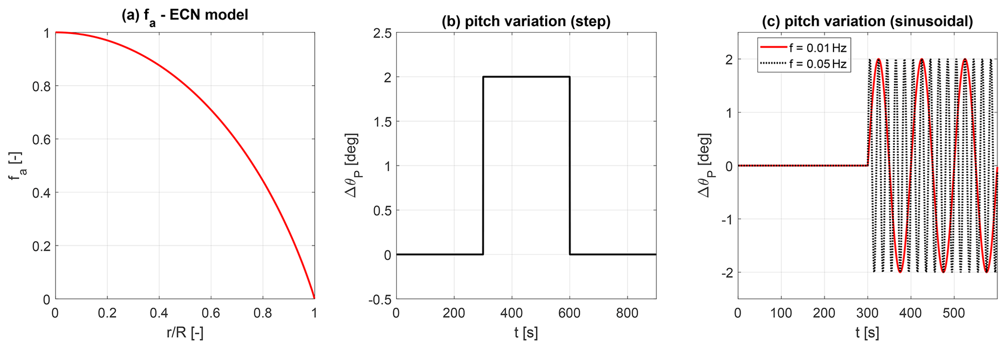
Figure 2 Radial evolution of the ECN model parameter f_a (a); blade pitch time history for the pitch step case (b); blade pitch time history for the two sinusoidal pitch cases (c).

3.1 Near-rated pitch steps

Blade pitch steps represent the traditional test case to investigate the performance of dynamic inflow models (e.g. Snel and Schepers, 1994; Sørensen and Madsen, 2006; Berger et al., 2020). This is because the slow response of the induction to sudden pitch changes leads to load overshoots that may affect the fatigue life of components. These pitch variations are often designed to be representative, at least to some extent, of fast controller actions.

A pitch step case has been considered in this work as well. The test selection has been inspired by a numerical case simulated in the international code comparison round of IEA Task 29 (Boorsma et al., 2018), where a very fast pitch variation was imposed on the AVATAR turbine. The very same pitch step variation has been prescribed in this case, starting from the design blade pitch value, suddenly raising it by 2^∘ towards feathering, holding it for 300 s, and finally returning to the initial condition (Fig. 2b) with a maximum pitch rate of ±10^∘ s⁻¹. The fast pitching rate helps highlight differences between the models.

The test has been run near rated conditions (10 m s⁻¹ wind speed) where dynamic inflow effects are expected to be most significant. Indeed, pitch control actions only start occurring once the rated power is reached, but the higher the wind speed, the lower the induction factor, leading to weaker dynamic wake effects. Therefore, the only standard operating region where pitch actions are likely to occur at high rotor induction (typically close to the Betz optimum) is the one near rated power. Rotational speed variations below rated conditions might also play a role, but they are usually much slower due to the great inertia of large variable-speed rotors and thus trigger few dynamic wake effects.

In order to isolate the unsteady behaviour from discrepancies in the steady-state values (always present between BEM and AWSM results, albeit small), the time histories of all quantities have been normalized as follows:

$$\begin{array}{}\text{(9)}& X^{*}\left(t\right)={\displaystyle \frac{X\left(t\right)-X_{\mathrm{0}{}^{\circ }}}{X_{\mathrm{0}{}^{\circ }}-X_{\mathrm{2}{}^{\circ }}}},\end{array}$$

with X(t) being the time history of a generic quantity, $X_{\mathrm{0}{}^{\circ }}$ and $X_{\mathrm{2}{}^{\circ }}$ the steady-state values before and after the feathering step, and X^*(t) the resulting normalized time history. Despite the normalization helping to better compare the results of different models, the radial dependency of the induction time histories hinders a synthetic visualization.

The axial induction responses, normalized via Eq. (9), at four spanwise locations are shown in Fig. 3. As expected, the ECN model predictions provide the worst match with AWSM, with the single time constant leading to a faster induction reconfiguration in both pitch step directions, which confirms the findings of previous studies (e.g. Boorsma et al., 2018; Pirrung and Madsen, 2018; Yu et al., 2019). This is especially true in the tip region where f_a approaches zero (Fig. 2a) and the ECN model response tends to be quasi-steady. Slightly better predictions have been obtained with the Øye model, which gives similar results to the ECN model in the inboard part of the blade but finds a slower decay close to the tip. The TUD-VR and DTU models provide the best match with AWSM for the case considered. Their predictions appear to be almost equivalent and both very similar to the free-vortex results until the blade tip, where a slightly faster decay than AWSM is observed. It is important to notice that, due to the very fast pitch rate, the AWSM results show a sudden spike in the induction response immediately after the step (i.e. around 300 and 600 s) that cannot be replicated by the BEM models. Section 3.1.1 shows this behaviour to be a result of the sudden change in the blade bound circulation induced by the pitch manoeuver, which produces strong shed vorticity in the near wake.

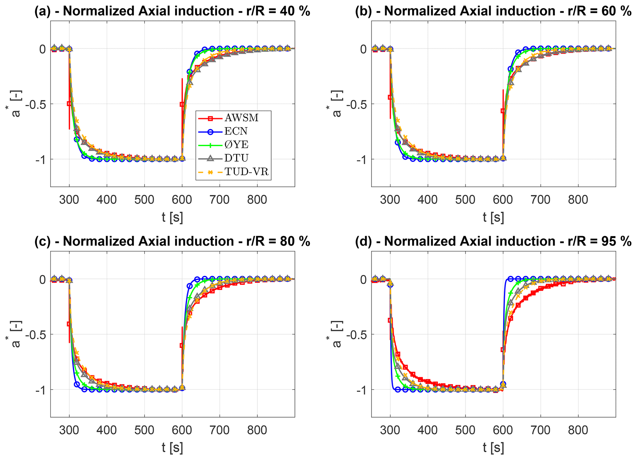
Figure 3 Normalized axial induction factor response to the pitch steps near rated conditions at four different radial locations: (a) 40 % span, (b) 60 % span, (c) 80 % span, and (d) 95 % span.

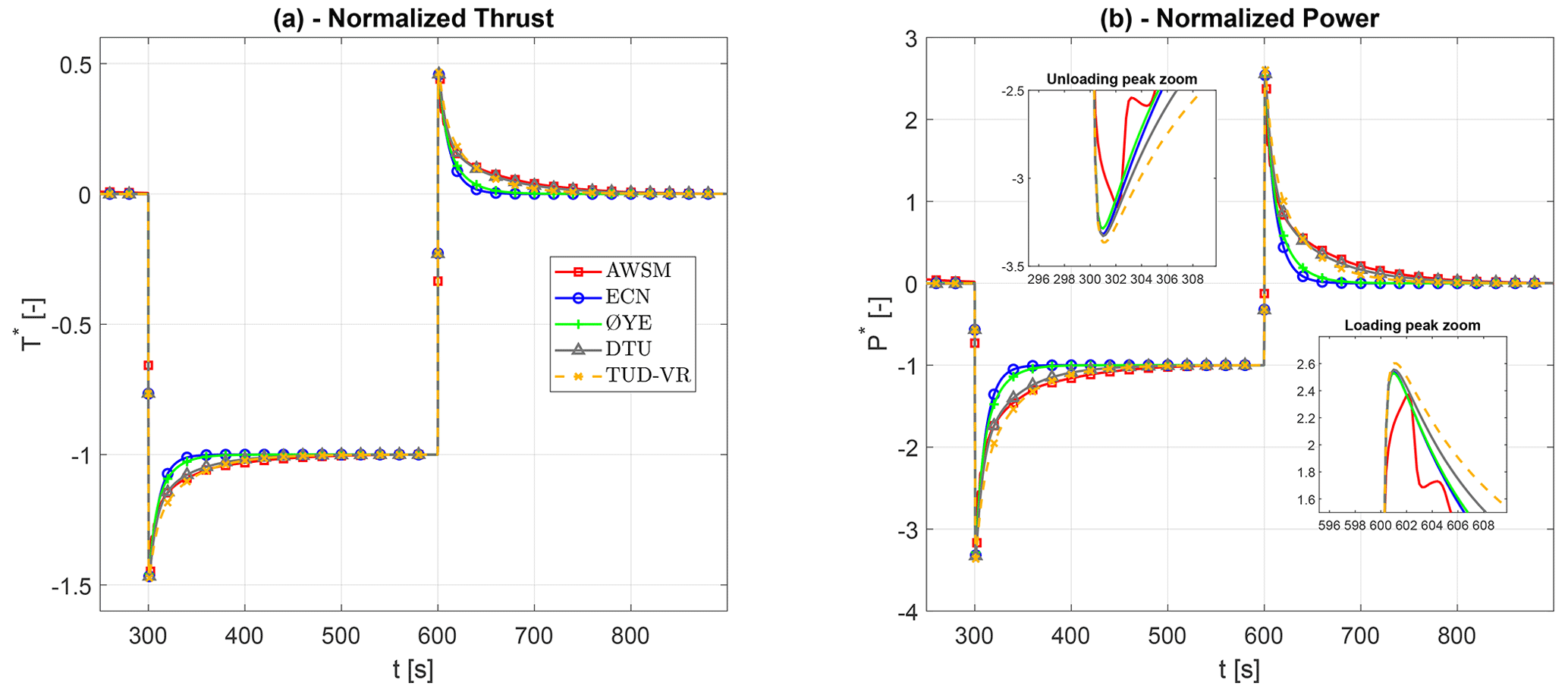
Figure 4 Normalized rotor aerodynamic thrust (a) and power (b) response to the blade pitch steps near rated conditions.

The normalized aerodynamic rotor thrust and power are plotted in Fig. 4. Their behaviour is consistent with the observations made on the induction field, with Øye and ECN models predicting a faster decay after the overshoot than TUD-VR, DTU, and AWSM. All BEM models slightly overestimate the overshoot peak, especially in terms of power where peaks are larger, and have been highlighted with small zoomed-in windows in Fig. 4b. This is a direct consequence of the induction spike caused by the shed vorticity that sharply increases the instantaneous induction right after the step and hence reduces and delays the overshoot.

3.1.1 The shed vorticity effect

As discussed in the previous section, a sudden peak in the induction response right after the pitch step and before the start of the exponential build-up has been observed. Zooming in around the time interval of the loading step reveals that thrust and power responses exhibit a staircase behaviour (Fig. 5c and d) similar to the one observed in IEA Task 29 that simulated pitch steps on the AVATAR turbine (Boorsma et al., 2018). To build on what was observed back then, a special AWSM version disregarding the shed vorticity contribution in all induced-velocity calculations has been developed. Although neglecting the presence of shed vortices violates Helmholtz's second theorem on vorticity, this special AWSM version is only used in comparison with the standard one, allowing us to highlight the impact of the shed vortices in the wake.

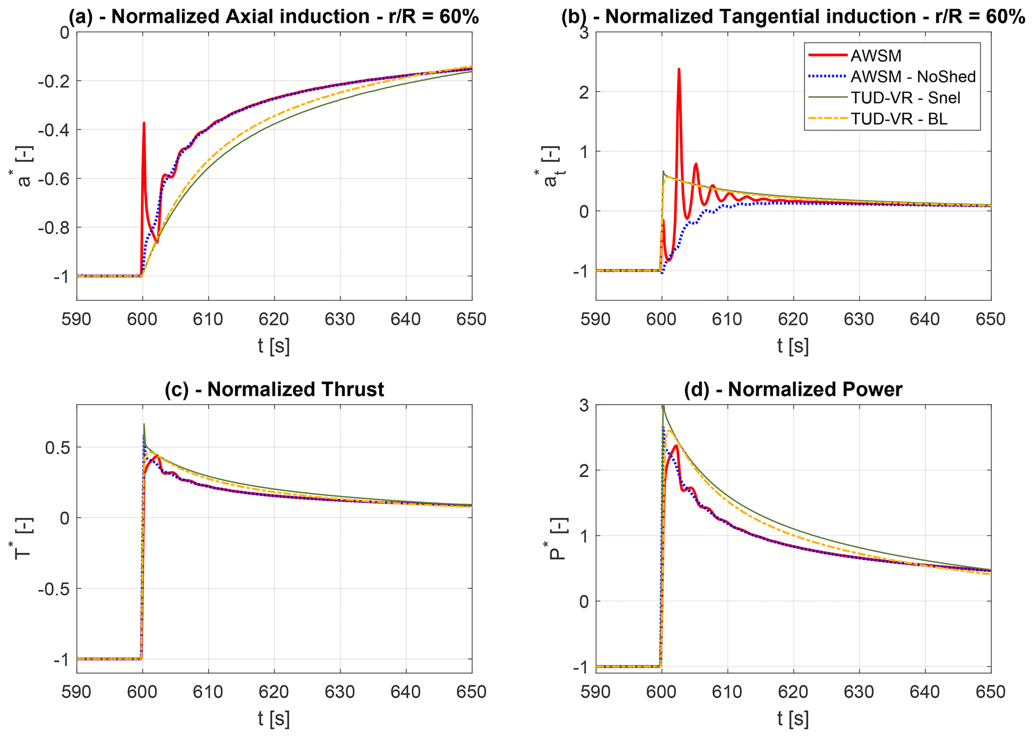
Figure 5 Zoomed-in view of the time interval near the loading step to highlight the effect of shed vorticity in the time history of (a) the normalized axial induction at 60 % span, (b) the normalized tangential induction at 60 % span, (c) the normalized aerodynamic thrust, and (d) the normalized aerodynamic power.

The plots in Fig. 5 also include the TUD-VR results obtained with two different dynamic stall models: the Beddoes–Leishman model (Hansen et al., 2004), which takes the Theodorsen effect on airfoils into account, and the Snel first-order model (Snel, 1997), which does not. This allows assessing the impact on induction results of modelling the shed vorticity at an airfoil level. Such a comparison is synthesized in Fig. 5, where the normalized axial and tangential induction factors at 60 % of the span are shown as an example (Fig. 5a and b), along with the normalized rotor thrust and power (Fig. 5c and d). Here it is noted that for these operating conditions and the spanwise location, the pitch step results obtained using Snel's first-order model are almost equivalent to those obtained without any dynamic stall model, and the latter results have not been reported for the sake of readability.

The axial induction plot clearly shows that without shed vorticity, the peak disappears and the staircase effect becomes less pronounced. This is even more evident in the tangential induction plot. In agreement with Task 29 findings, the lack of shed vorticity translates into a greater and earlier load overshoot (visible in Fig. 5c and d). Concerning the BEM results with the two dynamic stall models, it appears that the shed vorticity contribution in the Beddoes–Leishman model moves the predictions in the right direction, partially reducing and delaying the load overshoot as expected. However, this effect is much smaller than what is observed in AWSM, partly because the Beddoes–Leishman correction, in its current implementation, is only applied to the airfoil coefficients and only indirectly affects the induced velocities. Applying a shed vorticity correction to the induced velocities may improve the results, but such an investigation is left for future research. Another aspect contributing to the observed discrepancy is that the vortex shedding is modelled in a 2D fashion in BEM (using the Beddoes–Leishman model) assuming radial independence for each annulus. In other words, each airfoil is only affected by its own shed vorticity and is blind to what happens in the neighbouring elements. Whenever highly unsteady conditions are concerned, this approximation is expected to make the overall shed vorticity effect in BEM less significant than in reality, since only the airfoil scale is modelled.

One more interesting remark can be made by observing the tangential induction plot (Fig. 5b). The BEM models predict a small overshoot right after the pitch step, which is purely an effect of the coupling between axial and tangential momentum equations; i.e. correcting the quasi-steady axial induction leads to a new tangential induction value that guarantees a new equilibrium (Sect. 2.3). A tangential induction peak was also observed experimentally by Berger et al. (2021), and a similar trend can be recognized in the AWSM results as well once the initial oscillations induced by the shed vorticity are damped out. Although not reported here, the simulation of a slower pitch step where shed vorticity effects were negligible has produced similar tangential induction results for both BEM and AWSM, confirming the presence of a peak that compensates for the lower axial induction immediately after the pitch action.

3.2 Sinusoidal pitch variations

One of the main drawbacks of considering pitch steps to verify the performance of different dynamic inflow models is the difficulty of visualizing results in a compact yet comprehensive way. Prescribing sinusoidal collective blade pitch variations helps a lot in that sense. Observing that the spectrum of the induction response to a mono-harmonic blade pitch variation is dominated by the component at the pitch actuation frequency, the resulting unsteady axial induction can be fully characterized by the amplitude and phase of that harmonic. This allows characterizing all radial locations in one pair of plots.

Sinusoidal variations were also considered by Yu et al. (2019), but there the use of a uniformly loaded actuator disc allowed a direct prescription of the thrust coefficient variations. Here more detailed lifting-line rotor models are considered instead; therefore the rotor loading is only varied indirectly through the blade pitch angle. Due to the non-linear dependency of C_T on the blade pitch angle (especially at high loading) and the non-uniform spanwise loading of a real rotor, the present results are hardly comparable to those of Yu et al. (2019) though some conclusions are alike.

Both near- and above-rated conditions have been considered in this case, with wind speeds of 10 and 15 m s⁻¹ and average angles of attack of ∼7 and ∼4^∘, respectively. A sinusoidal blade pitch variation with respect to the design pitch setting has been prescribed, always with an amplitude of A_p=2^∘, which triggers significant dynamic wake effects while guaranteeing to avoid stall effects in the last 75 % of the blade span. Two different frequencies have been considered: f_p=10 and f_p=50 mHz. These correspond to a reduced rotor frequency (defined as $k=\frac{f_{\mathrm{p}}R}{V_{\mathrm{0}}}$, with f_p being the pitch frequency, R the rotor radius, and V₀ the free-stream wind speed) of k≃0.11 and k≃0.55 near rated conditions and k≃0.07 and k≃0.36 above rated conditions. The frequencies have been selected as multiples of the simulation time step to prevent leakage effects in the spectra that have been obtained via fast Fourier transform (FFT).

The near-rated results for the two pitch frequencies are shown in Figs. 6 and 7, respectively. The first plot in the two figures (Figs. 6a and 7a) shows the spanwise evolution of the reduced airfoil frequency (defined as $k_{\mathrm{airfoil}}=\frac{\mathit{\pi }{f}_{\mathrm{p}}c}{W}$, with f_p being the pitch frequency, c the airfoil chord, and W the airfoil effective wind speed). The mean effective wind speed found by AWSM during a pitch cycle has been used to compute k_airfoil. Even in the higher-frequency case, the values remain below the conventional 5% threshold from 25 % span onwards, with maximum values at the root never exceeding 10 %. This guarantees that unsteady airfoil effects are limited and standard polars can be relied upon in all the cases considered.

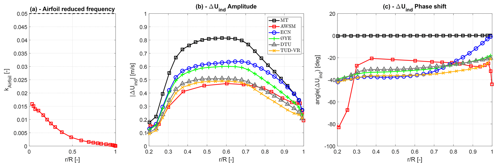
Figure 6 Spanwise distributions for the 10 mHz sinusoidal pitch variation near rated conditions (a) of the reduced airfoil frequency; (b) of the axial induced-velocity variation amplitude at the blade pitch frequency; and (c) of the axial induced-velocity variation phase at the blade pitch frequency, with respect to the phase of the prescribed pitch time series.

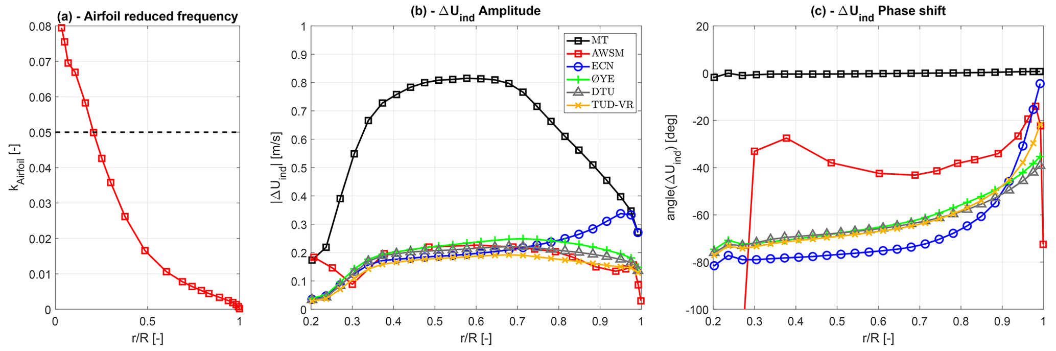
Figure 7 Spanwise distributions for the 50 mHz sinusoidal pitch variation near rated conditions (a) of the reduced airfoil frequency; (b) of the axial induced-velocity variation amplitude at the blade pitch frequency; and (c) of the axial induced-velocity variation phase at the blade pitch frequency, with respect to the phase of the prescribed pitch time series.

Figure 8 Spanwise distributions for the 50 mHz sinusoidal pitch variation above rated conditions (a) of the reduced airfoil frequency; (b) of the axial induced-velocity variation amplitude at the blade pitch frequency; and (c) of the axial induced-velocity variation phase at the blade pitch frequency, with respect to the phase of the prescribed pitch time series.

Looking at the amplitude-versus-span plots for the two frequencies (Figs. 6b and 7b), it can be noticed how dynamic inflow effects reduce the axial induced-velocity oscillations with respect to the quasi-steady momentum theory prediction (the black line in the figures), especially for the higher pitch frequency. Compared to AWSM, ECN and Øye models tend to slightly overestimate the oscillation amplitudes at the lower frequency (Fig. 6b). A better agreement is found for the faster pitch variation (Fig. 7b), except for the ECN model prediction in the outboard sections, which rises to reach the quasi-steady value at the tip. As in the pitch step case, the TUD-VR and DTU models provide very similar results that match the AWSM predictions well.

Figures 6c and 7c show the radial distribution of the phase shift between the axial induced-velocity oscillation (at the pitching frequency) and the blade pitch actuation signal. This phase shift was evaluated by considering the difference between the pitch frequency harmonic in the phase spectrum of the local induced-velocity signal (evaluated via FFT) and the phase of the sinusoidal blade pitch variation prescribed. Greater differences can be observed in these plots, with an average phase difference with respect to AWSM of about 30^∘ throughout the span for the fast-frequency case. Smaller discrepancies are also noticeable for the slower pitch variation. Besides the ECN line that always goes to zero at the tip (i.e. quasi-steady behaviour), the discrepancies between AWSM and the other BEM models are not fully understood. Searching for the critical parameters affecting such a phase shift, it was found that a reduction in the far-wake correction in the TUD-VR and DTU models generally improves the phase match with AWSM, although with conflicting effects on the amplitude (Schepers et al., 2021b). Shed vorticity also contributes to the observed phase differences, tending to reduce the phase delay in AWSM (as discussed in Sect. 3.2.1) and thus increasing the mismatch with BEM results.

Very similar conclusions can be drawn from the above-rated simulations. The slower blade pitch results have not been reported here, as dynamic inflow effects were barely visible due to the low rotor loading. The usual plots for the higher-frequency case of the above-rated simulations are shown in Fig. 8. As expected, the quasi-steady induction variation amplitudes are smaller than the corresponding near-rated case, leading to milder dynamic wake effects (Fig. 8b). In terms of model performance, the comments made for the rated case apply to these results as well, with all two-constant models behaving similarly and overestimating the phase shift compared to AWSM.

3.2.1 Shed vorticity effect

Similarly to the pitch step case, additional simulations have been carried out to investigate the effects of shed vorticity on the induction response to sinusoidal pitch variations. Only the higher-frequency case was considered, since the intensity of shed vortices grows with the pitch rate. Moreover, results are shown for the above-rated conditions, where controller-induced blade pitch corrections are more frequent and significant.

Figure 9 Effect of the shed vorticity on the 50 mHz sinusoidal pitch variation above rated conditions (a) on the distribution of the axial induced-velocity variation amplitude at the blade pitch frequency and (b) on the distribution of the axial induced-velocity variation phase at the blade pitch frequency, with respect to the phase of the prescribed pitch time series.

The corresponding amplitude and phase plots are shown in Fig. 9. As for the pitch step, the BEM lines (with the TUD-VR model for dynamic inflow) accounting or not accounting for shed vorticity in the dynamic stall model have been added, along with those of AWSM with and without shed vorticity. Figure 9a shows how shed vortices tend to slightly reduce the induced-velocity variation amplitude throughout the span, whereas in terms of phase, the no-shed vorticity line shows a larger (i.e. more negative) phase shift coming closer to the BEM predictions.

Switching between Snel and Beddoes–Leishman dynamic stall models to include the Theodorsen effect on the airfoil coefficients barely affects the BEM results, with minor differences noticeable in the inboard part of the blade only. Despite their very small extent, these discrepancies are a bit puzzling because unlike the pitch step case of Sect. 3.1.1, where the use of the Beddoes–Leishman model improved the match with the standard AWSM, here contrasting effects are observed for the amplitude and the phase. Furthermore, using the Snel model appears to have an opposite effect on the BEM predictions compared to neglecting the shed vorticity contribution in AWSM. A possible reason contributing to this inconsistency might be an unwanted effect of the Snel model that was found by Boorsma and Caboni (2020). When the airfoil lift curve deviates from the theoretical potential-flow slope, the model slightly acts in attached flow regions where it should not.

3.3 Impact of dynamic inflow models on the BEM results for DLC 1.2

To assess the impact of the different dynamic inflow models for BEM on a practical design load case, the procedure outlined in Sect. 2.4.2 has been followed. With DLC 1.2 being a fatigue load case, the main load time histories have been transformed into 1 Hz equivalent load cycles (Hendriks and Bulder, 1995) following the guidelines of IEC 61400-1. Figure 10 shows a comparison of the equivalent out-of-plane bending, in-plane bending, and torsion moments at the root of blade 1, along with the tower base fore–aft moment for several wind speeds along the turbine operating curve. The values have been normalized by the corresponding equivalent moments obtained by running steady-state BEM simulations (MT), i.e. without dynamic inflow models. This helps highlight the relative differences in various operating conditions.

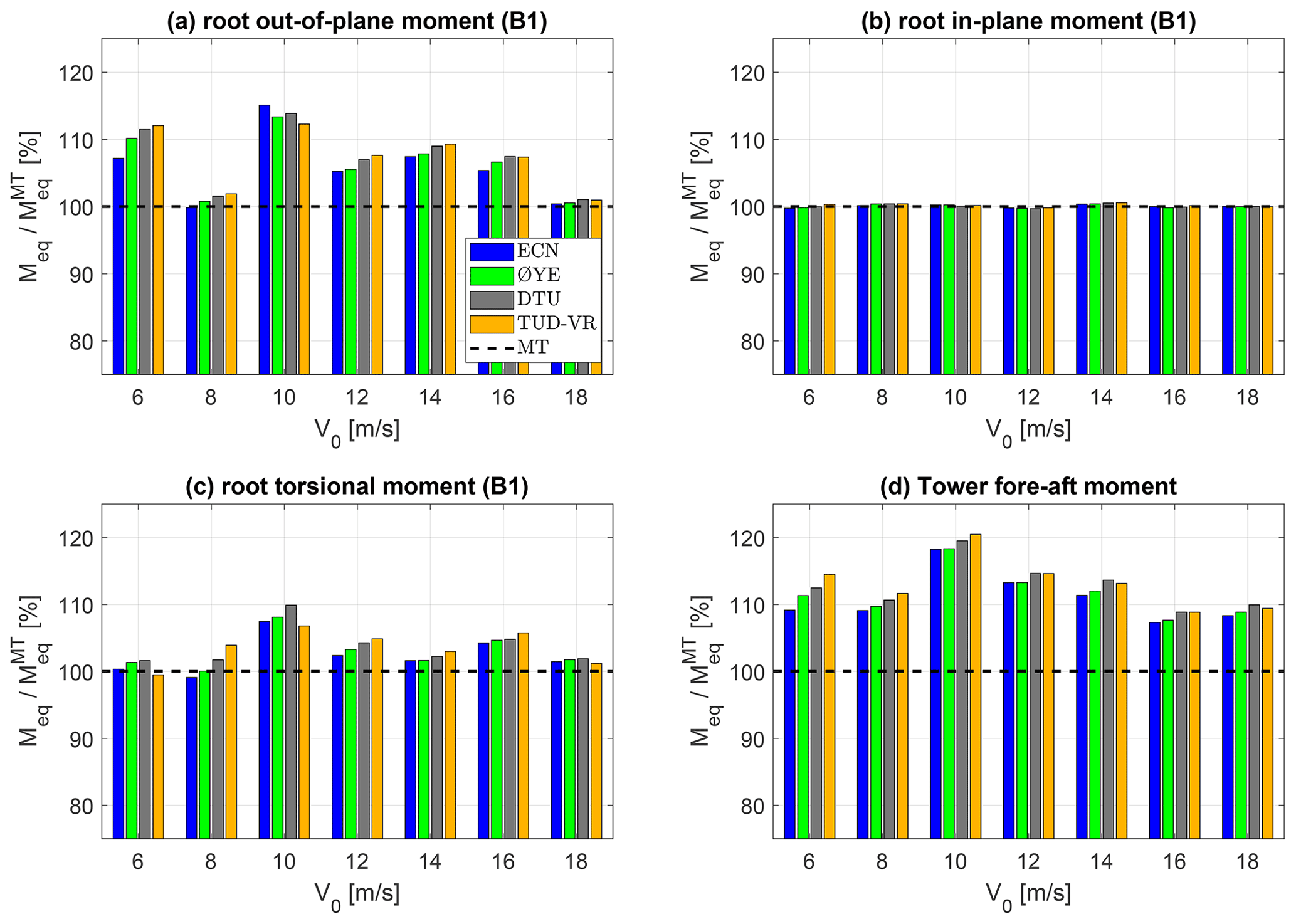
Figure 10 Comparison of 1 Hz equivalent moments obtained with the different dynamic inflow models for different wind speeds in DLC 1.2. The equivalent out-of-plane (a), in-plane (b), and torsional (c) moments at the root of blade no. 1 are reported along with the fore–aft moment at the tower base (d). All equivalent moments are normalized by the value obtained without using dynamic inflow models (MT).

In general, the use of a dynamic inflow model leads to higher equivalent loads of up to ∼10 % for the out-of-plane blade root bending moment (Fig. 10a). The tower base moment (Fig. 10d), which is driven by the rotor thrust and thus includes the contributions of all the blades, shows up to ∼20 % greater loads. Lower increments are observed in the equivalent torsion moment at the root of blade 1 as well (Fig. 10c). In contrast, the in-plane root bending moment (Fig. 10b) is almost insensitive to the dynamic inflow models as it is largely dominated by gravitational load cycles.

Provided that similar wind speed, rotor speed, and blade pitch time histories have been prescribed, the general equivalent load increase can be attributed to the damping of the induced-velocity fluctuations that results in greater aerodynamic load variations when dynamic inflow models are considered. The maximum equivalent load increase is always located around rated conditions (at 10 m s⁻¹ in this case) because this is where the blade pitch regulation starts and the rotor loading is still high. As the wind speed increases above rated conditions, the average induction lowers, leading to milder dynamic wake effects despite the relevant blade pitch regulation. The opposite is true below rated conditions, where the high tip speed ratio makes the rotor more sensitive to dynamic wake effects but the constant blade pitch reduces the chances of sharp loading variations occurring. In fact, unless considerable wind gusts occur, the large inertia of a more than 200 m diameter rotor makes rotational speed variations less prone to triggering strong dynamic inflow effects.

Provided that a dynamic inflow model is used in the BEM simulations, the choice of the specific model seems to matter significantly less in terms of equivalent load predictions. The differences found among the models always fall within 5 %, with larger discrepancies found at the wind speeds where the induction is higher. The TUD-VR and DTU models yield similar predictions to in the uniflow inflow cases (Sect. 3.1 and 3.2), with the Øye model typically falling between those and the ECN model results.

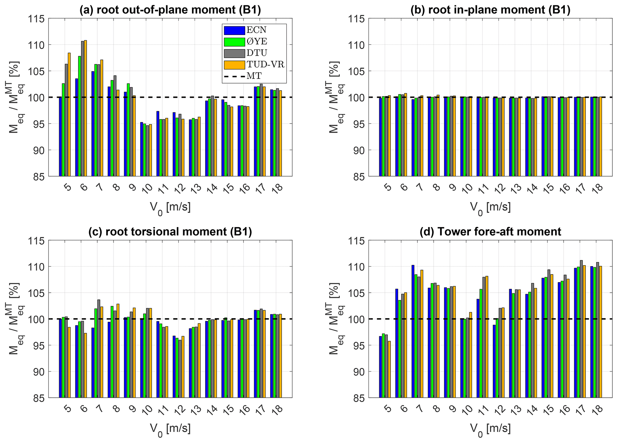
Once more, these results have been obtained by prescribing the time histories of the rotor operating conditions to aid their interpretation. The actual differences for a fully realistic load case including the original turbine controller and considering six seeds per wind speed have been found to be higher, especially below rated conditions (as shown in Fig. B1). This is because different dynamic inflow models lead to different controller actions and thus different operating conditions.

4 Conclusions

As part of the aerodynamic modelling activities in the TKI STRETCH project, three new dynamic inflow models have been implemented in AM's BEM solver: the Øye, the DTU, and the TUD-VR model. With these two-time-constant models, alternatives to the ECN model originally in AM, all the main dynamic inflow models available in the literature have been implemented. Sharing the same BEM solver and a common implementation strategy (Sect. 2.3) has reduced the uncertainty in the comparison of the different model predictions.

A 220 m diameter state-of-the-art offshore wind turbine designed in the STRETCH (2023) project has been considered for this comparative study. To facilitate the results' verification against free-vortex wake model predictions, a rigid rotor model in axial uniform inflow conditions has been considered first, prescribing conventional blade pitch steps as well as sinusoidal pitch variations. The latter offered a convenient way to visualize and compare the results. The effect of the blade shed vorticity on these uniform inflow cases has been investigated by exploiting a special version of AWSM, which neglects the contribution of shed vortices in the induced-velocity calculations.

Analysing fast pitch steps near rated conditions (Sect. 3.1) has shown that two-constant dynamic inflow models reproduce the induction decay better than the ECN model, especially in the blade tip region, confirming the conclusions of previous studies (e.g. Schepers, 2007; Sørensen and Madsen, 2006; Pirrung and Madsen, 2018). In this study, the best agreement with the free-vortex-wake results for the whole blade span has been reached with the most recent TUD-VR and DTU models that have been found to yield very similar predictions. The Øye model results typically fell between those and the ECN model predictions overestimating the speed of the induction recovery.

The free-vortex-wake results revealed a sudden induction peak occurring immediately after the fast pitch step, which reduces and delays the load overshoots/undershoots as observed by Boorsma et al. (2014). The comparison of AWSM results with and without wake shed vorticity has confirmed this axial induction peak to be a result of the strong vortices shed because of the sudden change in bound circulation induced by the pitch step, whereas the trailed vorticity only causes a slight staircase effect due to the finite number of blades. For the pitch steps, modelling shed vorticity effects on the airfoil coefficients with the Beddoes–Leishman model has been shown to improve BEM predictions but to a marginal extent compared to what the AWSM results with and without shed vorticity have highlighted.

The tangential induction response has been shown to be even more sensitive to the wake shed vorticity that, for the fast pitch step considered, caused strong oscillations in the AWSM results. A slight tangential induction peak, occurring right after the pitch step, has also been observed in BEM simulations. This is a consequence of the coupling between the axial and tangential BEM equations. By simulating a slower pitch step inducing weaker shed vortices, the presence of a similar peak has been confirmed by free-vortex simulations too, in agreement with recent experimental evidence from Berger et al. (2021).

The sinusoidal blade pitch variation cases have yielded similar findings to the pitch steps, highlighting the ECN model's tendency towards a quasi-steady behaviour near the blade tip. In terms of the induced-velocity variation amplitudes, two-constant models (especially TUD-VR and DTU) have provided quite accurate predictions for all the cases considered. For the phase, large discrepancies between BEM and AWSM results have been found in the fast-actuation cases instead. The use of AWSM with and without shed vorticity has shown these discrepancies to be partly caused by the shed vorticity, although, unlike the pitch step case, the use of the BL model has not improved the BEM predictions, leaving this point open to further investigations.

For the first time, the impact of dynamic inflow models on a fatigue design load case has been assessed quantitatively. Prescribing the same operating-condition time histories to guarantee a fair comparison, a systematic increase in the equivalent loads with respect to a steady-state BEM formulation has been found with all dynamic inflow models. The hypothesis of dynamic inflow effects being most relevant around rated wind conditions, where blade pitching occurs at high induction, has been confirmed, showing a 10 %–20 % increase in the 1 Hz equivalent out-of-plane bending moment at both the blade root and the tower base. Differences among the dynamic inflow models have been found to be larger at high rotor loading but always within 5 %. A more realistic comparison including the turbine controller has revealed larger discrepancies between the models, but the differences in operating conditions hinder the interpretation of the results (Appendix B).

Overall, this work has confirmed the superiority of two-constant models compared to the ECN model, for both the better modelling of the induction decay and the easier implementation in an implicit BEM, which avoids local convergence issues in non-uniform inflow conditions. The targets mentioned in Sect. 1 have been reached. However, concerning the ultimate goal of improving the accuracy of BEM design load calculations, this study suggests that further fine-tuning of the dynamic inflow models, albeit possible, is expected to have limited impact compared to improvements in the treatment of non-uniform inflow conditions or in the modelling of shed vorticity effects. Therefore, these aspects shall be given priority in future works. The next step for this dynamic inflow modelling activity will be the implementation of the recently proposed Øye model modification that improves the modelling of wind-gust-driven dynamic wake effects (Berger et al., 2022). Simulating DLC 1.2 with this new model may give a better idea of the relevance of turbulent wind variations for dynamic inflow effects on large rotors.

Appendix A: New dynamic inflow models' implementation

Nomenclature.
AM	TNO's library of aerodynamic solvers
	AeroModule (Boorsma et al., 2011)
AWSM	Aerodynamic Wind turbine Simulation
	Module – the free-vortex-wake module
	part of AM (van Garrel, 2003)
BL model	Beddoes–Leishman dynamic stall
	model (Hansen et al., 2004)
DTU model	dynamic inflow model for BEM
	presented by Madsen et al. (2020)
ECN model	dynamic inflow model for BEM
	developed by Snel and Schepers (1994)
MT	BEM implementation based on the
	classical momentum theory without a
	dynamic inflow model
Øye model	dynamic inflow model for BEM
	developed by Øye (1990)
Snel model	first-order dynamic stall model by
	Snel (1997)
TUD-VR	dynamic inflow model for BEM
	developed by Yu et al. (2019), calibrated
	with free-vortex-wake ring simulations

This appendix reports the expressions for the induced-velocity correction used by the different two-constant dynamic inflow models that have been implemented in AM as described in Sect. 2.3. The expressions for each dynamic inflow model are presented in the following sections.

A1 Øye model correction

The Øye model correction is computed with the following steps.

1. Evaluate the time constants ${\mathit{\tau }}_{{\mathrm{1}}_j}^t({\stackrel{\mathrm{‾}}{a}}_{Q{S}_j}^t,{\stackrel{\mathrm{‾}}{V}}_{{\mathrm{0}}_j}^t)$ and ${\mathit{\tau }}_{{\mathrm{2}}_j}^t({\mathit{\tau }}_{{\mathrm{1}}_j}^t,r_j)$ according to the expressions reported in Snel and Schepers (1994).

2. Evaluate $y_j^t$ solving Eq. (2) (with backward discretization).

3. Calculate the following Øye model correction (from Eq. 3):

   $$\begin{array}{}\text{(A1)}& \mathrm{\Delta }{u}_j^t={\displaystyle \frac{y_j^t+\frac{{\mathit{\tau }}_{{\mathrm{2}}_j}^t}{\mathrm{\Delta }t}{\stackrel{\mathrm{‾}}{u}}_j^{t-\mathrm{1}}}{\mathrm{1}+\frac{{\mathit{\tau }}_{{\mathrm{2}}_j}^t}{\mathrm{\Delta }t}}}-{\stackrel{\mathrm{‾}}{u}}_{Q{S}_j}^t.\end{array}$$

Here it is noted that alternative implementation methods exist; e.g. Hansen (2015) proposed a different strategy based on analytical solutions of the ordinary differential equations. Similar implementation choices may affect the numerical stability of the code and may deserve further investigation. Nevertheless, no issues of numerical stability have been encountered in the simulations carried out in this work using the algorithms described in this appendix.

A2 TUD-VR model correction

The TUD-VR model correction is computed with the following steps.

1. Evaluate the local thrust coefficient $C_{T_j}^t\left({\stackrel{\mathrm{‾}}{a}}_{Q{S}_j}^t\right)$.

2. Evaluate the model parameters ${\mathit{\beta }}_j^t(C_{T_j}^t,r_j)$, ${\mathit{\omega }}_{{\mathrm{1}}_j}^t(C_{T_j}^t,r_j)$, and ${\mathit{\omega }}_{{\mathrm{2}}_j}^t(C_{T_j}^t,r_j)$ from the polynomial expressions reported in Yu et al. (2019).

3. Evaluate $c_{{\mathrm{1}}_j}^t$ and $c_{{\mathrm{2}}_j}^t$ solving Eqs. (5) and (6) (with backward discretization).

4. Calculate the following TUD-VR model correction (from Eq. 4):

   $$\begin{array}{}\text{(A2)}& \mathrm{\Delta }{u}_j^t=-{\displaystyle \frac{\mathrm{1}}{\mathrm{2}}}\left(c_{{\mathrm{1}}_j}^t+c_{{\mathrm{2}}_j}^t\right).\end{array}$$

A3 DTU model correction

The DTU model correction is computed with the following steps.

1. Compute the model parameters $f_{{\mathrm{1}}_j}^t\left({\stackrel{\mathrm{‾}}{a}}_{Q{S}_j}^t\right)$ and $f_{{\mathrm{2}}_j}^t\left({\stackrel{\mathrm{‾}}{a}}_{Q{S}_j}^t\right)$ and ${\mathit{\tau }}_{{\mathrm{1}}_j}^t\left(r_j\right)$ and ${\mathit{\tau }}_{{\mathrm{2}}_j}^t\left(r_j\right)$ from the expressions reported in Madsen et al. (2020).

2. Evaluate the following exponential filters: $E_{{\mathrm{1}}_j}^t=\exp \left(-\mathrm{\Delta }t\frac{{\stackrel{\mathrm{‾}}{V}}_{{\mathrm{0}}_j}^t}{R}\frac{f_{{\mathrm{1}}_j}^t}{{\mathit{\tau }}_{{\mathrm{1}}_j}^t}\right)$ and $E_{{\mathrm{2}}_j}^t=\exp \left(-\mathrm{\Delta }t\frac{{\stackrel{\mathrm{‾}}{V}}_{{\mathrm{0}}_j}^t}{R}\frac{f_{{\mathrm{2}}_j}^t}{{\mathit{\tau }}_{{\mathrm{2}}_j}^t}\right)$.

3. Evaluate the following DTU model correction:

   $$\begin{array}{}\text{(A3)}& \mathrm{\Delta }{u}_j^t=A_{\mathrm{1}}{Y}_{{\mathrm{1}}_j}^t+A_{\mathrm{2}}{Y}_{{\mathrm{2}}_j}^t-{\stackrel{\mathrm{‾}}{u}}_{Q{S}_j}^t,\end{array}$$

   with

   $$\begin{array}{}\text{(A4)}& {\displaystyle }& {\displaystyle }{A}_{\mathrm{1}}=\mathrm{0.5847},A_{\mathrm{2}}=\mathrm{0.4153},\text{(A5)}& {\displaystyle }& {\displaystyle }{Y}_{{\mathrm{1}}_j}^t=Y_{{\mathrm{1}}_j}^{t-\mathrm{1}}{E}_{{\mathrm{1}}_j}^t+{\stackrel{\mathrm{‾}}{u}}_{Q{S}_j}^t\left(\mathrm{1}-E_{{\mathrm{1}}_j}^t\right),\text{(A6)}& {\displaystyle }& {\displaystyle }{Y}_{{\mathrm{2}}_j}^t=Y_{{\mathrm{2}}_j}^{t-\mathrm{1}}{E}_{{\mathrm{2}}_j}^t+{\stackrel{\mathrm{‾}}{u}}_{Q{S}_j}^t\left(\mathrm{1}-E_{{\mathrm{2}}_j}^t\right).\end{array}$$

Note that $Y_{{\mathrm{1}}_j}^t$ and $Y_{{\mathrm{2}}_j}^t$ correspond to the parameters $u_{i,y,\mathrm{1}}^t$ and $u_{i,y,\mathrm{2}}^t$ defined in Madsen et al. (2020). The names have been changed to avoid confusion with the notation.

Appendix B: DLC 1.2 results with the official controller

Figure B1 shows the results of standard DLC 1.2 simulations featuring the official STRETCH turbine controller (including IPC). The plots are the same as in Fig. 10, but the average loads among six seeds are shown for a wider set of wind speeds. For each wind speed, the same random seeds were used for the different dynamic inflow models. The results' validity has been checked thoroughly, finding that the observed trends are well aligned with the standard deviations of both the operating quantities (i.e. blade pitch and rotor speed) and the loads. These differences are tightly linked to the controller behaviour. This makes their interpretation not only very difficult but also case specific, so the effect of each model on the equivalent loads might be hard to generalize from these results. The plot is anyhow left in this appendix for the interested reader to reflect upon.

Figure B1 Here the results obtained with the original controller considering six seeds per wind speed (only the average value among the seeds is plotted) are reported in similar plots to those shown in Fig. 10.