the Creative Commons Attribution 4.0 License.
the Creative Commons Attribution 4.0 License.
 | 24 Mar 2023
Comparison of free vortex wake and blade element momentum results against large-eddy simulation results for highly flexible turbines under challenging inflow conditions
Benjamin Anderson
Luis A. Martínez-Tossas
Emmanuel Branlard
Nick Johnson
Throughout wind energy development, there has been a push to increase wind turbine size due to the substantial economic benefits. However, increasing turbine size presents several challenges, both physically and computationally. Modeling large, highly flexible wind turbines requires highly accurate models to capture the complicated aeroelastic response due to large deflections and nonstraight blade geometries. Additionally, the development of floating offshore wind turbines requires modeling techniques that can predict large rotor and tower motion. Free vortex wake methods model such complex physics while remaining computationally tractable to perform key simulations necessary during the turbine design process. Recently, a free vortex wake model – cOnvecting LAgrangian Filaments (OLAF) – was added to the National Renewable Energy Laboratory's engineering tool OpenFAST to allow for the aerodynamic modeling of highly flexible turbines along with the aero-hydro-servo-elastic response capabilities of OpenFAST. In this work, free vortex wake and low-fidelity blade element momentum (BEM) results are compared to high-fidelity actuator-line computational fluid dynamics simulation results via the Simulator fOr Wind Farm Applications (SOWFA) method for a highly flexible downwind turbine for varying yaw misalignment, shear exponent, and turbulence intensity conditions. Through these comparisons, it was found that for all considered quantities of interest, SOWFA, OLAF, and BEM results compare well for steady inflow conditions with no yaw misalignment. For OLAF results, this strong agreement with the SOWFA results was consistent for all yaw misalignment values. The BEM results, however, deviated significantly more from the SOWFA results with increasing absolute yaw misalignment. Differences between OLAF and BEM results were dominated by the yaw misalignment angle, with varying shear exponent and turbulence intensity leading to more subtle differences. Overall, OLAF results were more consistent than BEM results when compared to SOWFA results under challenging inflow conditions.
- Article
(8202 KB) - Full-text XML
- BibTeX
- EndNote


The U.S. Government retains and the publisher, by accepting the article for publication, acknowledges that the U.S. Government retains a nonexclusive, paid-up, irrevocable, worldwide license to publish or reproduce the published form of this work, or allow others to do so, for U.S. Government purposes.
Over the years, wind energy researchers have focused on increasing wind turbine rotor size, yielding substantial reductions in wind energy costs. As rotor size increases, substantially more energy is captured through a greater swept area, thus increasing turbine capacity factor while reducing specific power. Low-specific-power rotors, with correspondingly higher capacity factors, have been shown to lead to higher economic value (Bolinger et al., 2021). One important consideration for such large turbines, however, is increased blade flexibility. In particular, large blade deflection likely results from large, highly flexible wind turbine blades. The dynamic and complex nature of large blade deflections leads to the violation of many assumptions used by common aerodynamic models, such as the blade element momentum (BEM) method. Such aerodynamic models are originally valid for axisymmetric rotor loads contained in a plane and for which there is little to no interaction between the turbine blades and the near wake of the turbine. When operating under normal conditions, large blade deflections may cause a swept rotor area that deviates significantly from the rotor plane and the turbine near wake to diverge from a uniform helical shape. The fact that the steady-state swept area deviates from a plane increases the three-dimensional interactions between the blade elements and therefore further violates the assumptions of blade annuli independence. The unsteady motion of the blade resulting from the increased flexibility of modern blade designs leads to large angle-of-attack fluctuations, meaning an accurate and robust dynamics stall model is important. Further, a nonuniform near wake increases interactions between turbine blades and the local near wake, thus violating assumptions of models that do not account for the position and dynamics of the near wake. In addition to the complications from large blade deflection, there are many other complex wind turbine situations that violate simple engineering assumptions. Such situations include accurately capturing aerodynamic loads for nonstraight blade geometries (e.g., built-in curvature or sweep); skewed flow caused by yawed inflow, turbine tilt, or strong shear; and large rotor motion caused by the placement of a turbine atop a compliant floating offshore platform.
Large, flexible rotors and complex operating conditions necessitate higher-fidelity aerodynamic models. By definition, computational fluid dynamics (CFD) methods are able to capture the necessary physics of such problems. However, the high computational cost limits the number of simulations that can be practically performed for a given problem, which is an important consideration in load analysis for turbine design. Free vortex wake (FVW) methods model the complex physics required for such problems while remaining less computationally expensive than CFD methods. Many FVW methods have been developed, ranging from the early treatments by Rosenhead (1931) and the formulation of vortex particle methods by Winckelmans and Leonard (1993) to the recent mixed Eulerian–Lagrangian compressible formulations of Papadakis (2014). Established FVW codes in wind energy include the vortex particle approach of GENUVP (Voutsinas, 2006) and the vortex filament approach of AWSM (van Garrel, 2003), both of which are coupled to structural solvers. The method was extended by Branlard et al. (2015) to use vortex methods in the aeroelastic modeling of wind turbines in sheared and turbulent inflow. The limitations of BEM were highlighted in previous studies that compared FVW and BEM (Hauptmann et al., 2014; Perez-Becker et al., 2020) or FVW and large-eddy simulations (Meyer Meyer Forsting et al., 2019). Vortex theory has been used to answer some of the shortcomings of BEM. Examples of corrections related to the independence of radial annuli, yaw, and tip losses are discussed in Branlard (2017). Corrections for out-of-plane deflections and coning are found in Li et al. (2022a, b). Yet FVW methods are now reaching a stage where they can be used for full load case calculations (Boorsma et al., 2020).
This work focuses on the FVW model that was recently implemented into the modeling tool OpenFAST (Shaler, 2020); cOnvecting LAgrangian Filaments (OLAF) is an FVW model used to compute the aerodynamic forces on moving two- and three-bladed horizontal-axis wind turbines. This module is incorporated into the National Renewable Energy Laboratory's (NREL's) physics-based engineering tool OpenFAST, which solves the aero-hydro-servo-elastic dynamics of individual wind turbines. OLAF is incorporated into the OpenFAST module AeroDyn15 as an alternative to the traditional BEM option. Incorporating the OLAF module into OpenFAST allows for the modeling of highly flexible turbines along with the aero-hydro-servo-elastic response capabilities of OpenFAST. Following discretization and regularization studies, the purpose of this work is to determine the accuracy of an aeroelastically coupled FVW method under conditions known to be challenging to lower-fidelity aerodynamic methods. This is done by comparing OLAF results to actuator-line large-eddy simulation via SOWFA and low-fidelity BEM results for a large range of yaw misalignment, shear exponent, and turbulence intensity (TI) conditions. These comparisons provide a better understanding of the relative performance of OLAF, BEM, and the actuator-line formulation of SOWFA (Churchfield et al., 2012) when subjected to a range of inflow conditions, both simple and challenging. Combined with the discretization and regularization studies, this will aid in the selection of the most appropriate modeling tool based on the application and available resources.
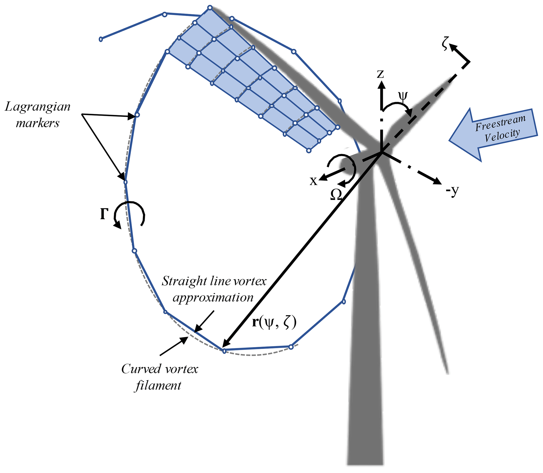
Figure 1Evolution of near wake lattice, blade-tip vortex, and Lagrangian markers. Note that the blade-root vortex is also present in the formulation but not shown in the figure.
2.1 Overview of OLAF
The OLAF module uses a lifting-line representation of the blades, which is characterized by a distribution of bound circulation. The spatial and time variation in the bound circulation results in free vorticity being emitted in the wake. OLAF solves for the turbine wake in a time-accurate manner, which allows the vortices to convect, stretch, and diffuse. The OLAF model is based on a Lagrangian approach, in which the turbine wake is discretized into Lagrangian markers. There are many methods of representing the wake with Lagrangian markers (Branlard, 2017). In this work, a hybrid lattice–filament method is used, as depicted in Fig. 1. Here, the position of the Lagrangian markers is shown in terms of wake age ζ and azimuthal position ψ, though in the code they are defined in terms of Cartesian coordinates. A lattice method is used in the near wake of the blade. The near wake spans over a user-specified angle. Though past research has indicated that a near wake region of 30∘ is sufficient (Leishman et al., 2002; Ananthan et al., 2002), it has been shown that a larger near wake is required for high thrust and other challenging conditions. This is further investigated in this work. After the near wake region, the wake is assumed to instantaneously roll up into root and tip vortices, which are assumed to be the most dominant features for the remainder of the wake (Leishman et al., 2002). Each Lagrangian marker is connected to adjacent markers by straight-line vortex filaments. The wake is discretized based on the spanwise location of the blade sections and a specified time step (dt), which may be different from the time step of AeroDyn15. The wake is allowed to move and distort with time, thus changing the wake structure as the markers are convected downstream. To limit computational expense, the root and tip vortices are truncated after a specific distance downstream from the turbine. The wake truncation violates Helmholtz's first law and hence introduces an erroneous boundary condition. To alleviate this, the wake is “frozen” in a buffer zone between a specified buffer distance and the wake length. In this buffer zone, the markers convect at the average ambient velocity, minimizing the truncation error (Leishman et al., 2002). The buffer zone is typically chosen as the convected distance over one rotor revolution.
As part of OpenFAST, induced velocities at the lifting line/blade are transferred from OLAF to AeroDyn15 and used to compute the effective blade angle of attack at each blade station, which is then used to compute the aerodynamic forces on the blades. The OLAF method returns the same information as the BEM method but allows for more accurate calculations in areas where BEM assumptions are violated, such as those discussed above. Unsteady aerodynamic effects, such as dynamic stall, are accounted when using OLAF using the same models as the BEM method of AeroDyn15, but the shed vorticity effect is removed when OLAF is used.
The governing equation of motion for a vortex filament is given by
where r is the position vector of a Lagrangian marker and V is the velocity. Vortex filament velocity is a nonlinear function of the vortex position, representing a combination of the freestream and induced velocities (Hansen, 2008). The induced velocities at each marker, caused by each straight-line filament, are computed using the Biot–Savart law, which considers the locations of the Lagrangian markers and the intensity of the vortex elements (Leishman et al., 2002):
where Γ is the circulation strength of the filament, dl is an elementary length along the filament, and r is the vector between a point on the filament and the control point x. The regularization factor Fν is introduced because of the singularity that occurs in the Biot–Savart law at the filament location (Vatistas et al., 1991). Viscous effects prevent this singularity from occurring. In this work the Vatistas regularization function is used, given by
where rc is the regularization parameter or vortex core radius. OLAF uses a different regularization value for the blades and the wake. Viscosity diffuses the vortex strength with time, which is modeled by increasing the wake regularization parameter using a “core-spreading” model, given by Eq. (4).
where α=1.25643, ν is the kinematic viscosity, ζ is the wake age, and δ is a core spread eddy viscosity parameter. Additional details and models are found in Shaler et al. (2020).
The circulation along the blade span is computed using a lift-coefficient-based method. This method determines the circulation within a nonlinear iterative solver that utilizes the polar data at each control point on the lifting line. The algorithm ensures that the lift obtained using the angle of attack and the polar data match the lift obtained with the Kutta–Joukowski theorem. This method is based on the work of van Garrel (2003) and is further detailed in the OLAF User's Guide and Theory Manual (Shaler et al., 2020).
2.2 Overview of SOWFA
The Simulator fOr Wind Farm Applications (SOWFA) is a collection of software libraries used to perform large-eddy simulations of wind plant flows (Churchfield et al., 2012; Churchfield and Lee, 2021). SOWFA is built on top of the OpenFOAM framework (Weller et al., 1998). In SOWFA, the spatially filtered Navier–Stokes equations are solved using a finite-volume formulation. The spatial derivatives are computed using second-order finite-difference, and the time advancing is done using second-order backward differentiation. The wind turbine blades and tower are modeled using body forces from the actuator-line model (Martínez-Tossas et al., 2015; Churchfield et al., 2015; Sørensen and Shen, 2002). Velocity sampling is done at the actuator points, to be consistent with the original formulation of the actuator-line model and other studies (Sørensen and Shen, 2002; Martínez-Tossas et al., 2015, 2018). The results presented use 50 actuator points along the blades and , following the work from Churchfield et al. (2017). The grid resolution of the background mesh was 0.91 D with two levels of local refinement to achieve a grid size of 0.023 D in the turbine location.
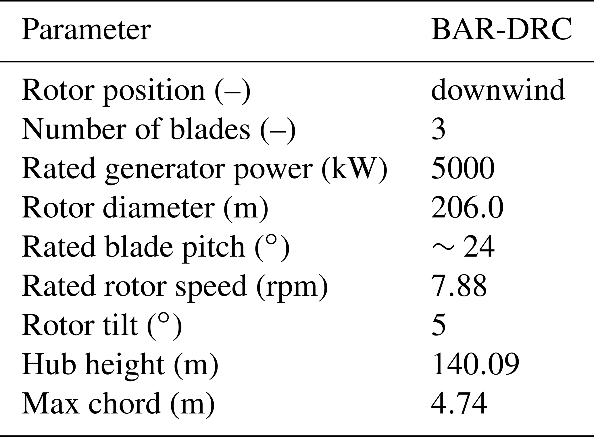
Table 2Wake parameter specification study ranges.
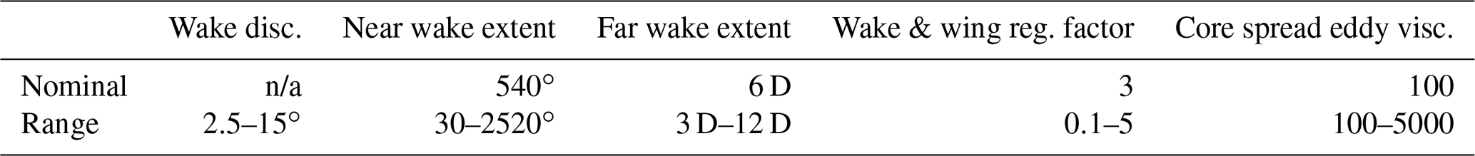
Note that n/a stands for not applicable.
2.3 Wake parameter specification study results
All studies were performed using the Big Adaptive Rotor (BAR) Downwind Rail Carbon (DRC) turbine (Bortolotti et al., 2021), described in Table 1, to determine recommended values for various OLAF input parameters. All cases were 10 min simulations – not including initial transients – with a set rotor speed and blade pitch. The studies were performed with uniform wind speeds ranging from 4 to 12 m s−1, with the ranges for each study shown in Table 2. The studies were done sequentially as presented here, meaning that the wake discretization study was the first to be completed, with the “nominal” values from Table 2 used for the remaining parameters considered in this work. From this study, an optimal wake discretization value was determined. This value was used as the wake discretization value for all remaining studies. The near wake extent study was performed next, using the optimal wake discretization value from the previous study and the remaining nominal values from Table 2. The optimal value determined from this study was used in the far wake extent study and so on. Output quantities of interest (QoIs) are summarized in Table 3. An overview of the results is included here; for detailed results, see the online OLAF documentation (Shaler et al., 2022).
Table 3Quantities of interest for discretization and regularization studies.
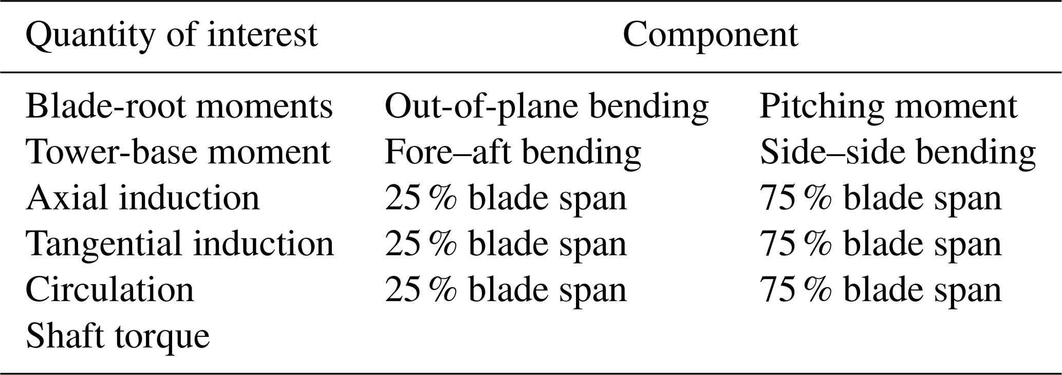
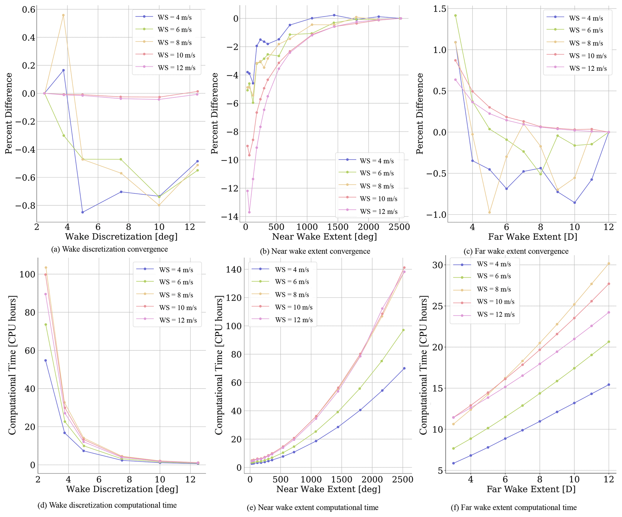
Figure 2(a–c) Percent differences and (d–f) computational time of time-averaged rotor power, varying for (a, d) wake discretization, (b, e) near wake extent, and (c, f) far wake extent. Each line color represents a different hub-height wind speed. Wake discretization results are relative to 2.5∘. Near wake extent results are relative to 2520∘ (seven revolutions). Far wake extent results are relative to 12 D. WS: wind speed.
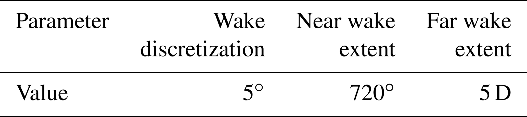
Table 4Recommended values selected from the results of the discretization and wake extent studies.
2.3.1 Wake discretization and extent
The wake discretization and extent convergence studies observed how wind turbine QoIs varied with changing wake discretization, near wake extent, and far wake extent. These are user-defined parameters for OLAF and are known to have a large effect on both wind turbine response and simulation time. The wake discretization is specified by the AeroDyn15 time step, using the equation . Because rotor speed is a turbine characteristic, dψ is defined using dt, which remains constant throughout the simulation. A smaller time step results in a finer wake discretization. The near wake extent is specified by the number of degrees to be used in the lattice near wake computations. The far wake extent is defined by specifying the wake length used in the tip- and root-vortex filaments calculations. By reducing the time step or increasing the wake length, the simulation accuracy is expected to improve, along with the computational expense. Accuracy is assessed by computing the percent difference of the mean QoI value at each test point relative to the finest or largest value for the discretization and wake extent studies, respectively. To balance model accuracy with computational cost, a convergence criteria of ∼2 %, was selected. The recommendations and computational costs in this section are based on all QoIs in Table 3. However, due to space constraints only generator power is shown. Other results can be seen in Shaler et al. (2022).
An optimal value was found across all wind speeds for each study, as reported in Table 4. Generator power convergence for each parameter is shown in Fig. 2a, b, and c. Computational time for variations in each parameter is shown in Fig. 2d, e, and f. All simulations are run using a tree-code algorithm with a time complexity 𝒪(nlog n). There is no clear convergence for the wake discretization study. Results for fine wake discretization are likely to be a function of the wake regularization factor, which is a topic requiring further research (see Sect. 2.3.2). Regardless, the percent difference remains below ±1 % for all discretization values. Therefore, the computational cost in Fig. 2d plays a large part in selecting the recommended discretization value. Based on these results, a wake discretization of 5∘ was selected as the optimal value. The near wake extent results in Fig. 2b show clear convergence with increasing wake length. This is expected, as a longer wake captures more induction at the rotor (see the discussion related to Fig. 3). From this plot, the necessary near wake length to meet the 2 % convergence criteria is a function of wind speed, with higher wind speeds requiring a longer wake. To ensure the criteria are satisfied for most wind speeds while remaining computationally tractable, a near wake length of 720∘ is recommended. Variability in relative error is observed for increased far wake extents at lower wind speeds in Fig. 2c, but the error generally decreases for longer far wakes. Despite this variation, percent difference remains below 2 % for all far wake lengths. This is likely due to the sufficient near wake length. Therefore, the far wake length recommendation is largely based on computational expense. Note that the values reported in Table 4 were deemed optimal for the specific wind turbine used in this paper under uniform inflow wind but are not necessarily optimal for other configurations. These results could vary based on turbine model and inflow condition, including the addition of turbulence, and can be varied based on accuracy and computational cost requirements. However, they can serve as a starting point for other systems and inflows.
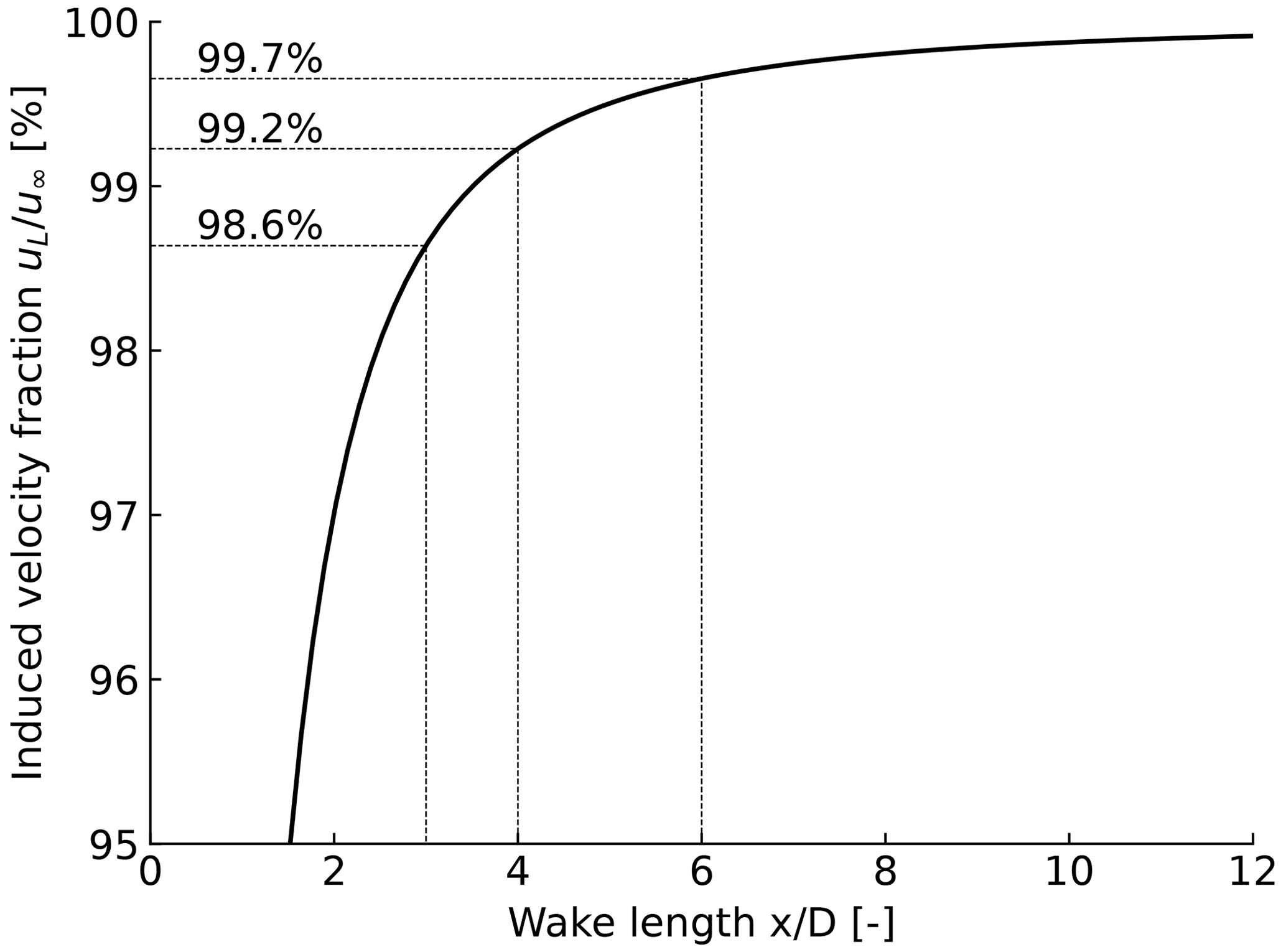
Figure 3Fraction of induced velocity for various wake length as obtained using vortex cylinders of finite and infinite lengths.
The wake length required for a given accuracy can be assessed by comparing the induced velocity at the rotor plane as obtained from a vortex cylinder of finite length (uL) and from a vortex cylinder of infinite length (u∞), the ratio of which is shown in Fig. 3. Both velocities can be obtained using closed-form formulae (Branlard and Gaunaa, 2014). It is seen that 99 % of the axial induction is provided by the first four diameters of the wake of a vortex cylinder. This observation supports the recommended value of 5 D selected in Table 4.
2.3.2 Regularization
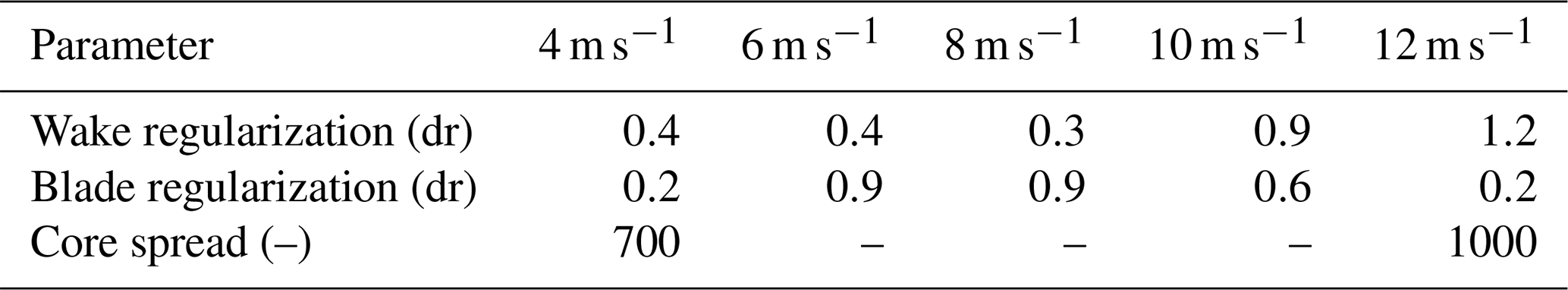
The wake regularization factor, blade regularization factor, and core-spreading eddy viscosity were examined for the regularization study. The method was the same as the wake discretization and extent studies, except that results were compared against those obtained using the actuator-line formulation of SOWFA (Churchfield et al., 2012) to determine the optimal parameter values. This was done because it is not possible to know a priori which regularization parameter can be used as a reference. A core-spreading value of 0.05 was used in SOWFA. This value is close to the typical values used in other studies but is not expected to produce optimal results (Martínez-Tossas et al., 2015; Martinez-Tossas et al., 2017; Churchfield et al., 2017; Martínez-Tossas et al., 2018). Recent work suggests that optimal results require much finer grid resolutions or advanced aerodynamic formulations (Martínez-Tossas and Meneveau, 2019; Meyer Forsting et al., 2019), which were not available for this study. Using an optimal regularization is an active research topic, and the question remains as to whether the actuator-line simulations can be used as a reference. With this in mind, the different parameter values found to minimize the difference with SOWFA for different wind speeds (i.e., zero crossing in Fig. 4) are reported in Table 5. Computational time was generally insensitive to these parameter values, so it is not reported. Time-averaged generator power results are shown in Fig. 4 for the wake regularization factor study. Based on the results given in Table 5, no clear trend is found between the regularization factors and the wind speed. It appears that a reasonable approximation would consist of setting the regularization parameters to 0.5 dr, where dr is the blade spanwise discretization. More research is nevertheless needed, both for actuator-line CFD and lifting-line-based codes, to find the optimal values of these parameters.
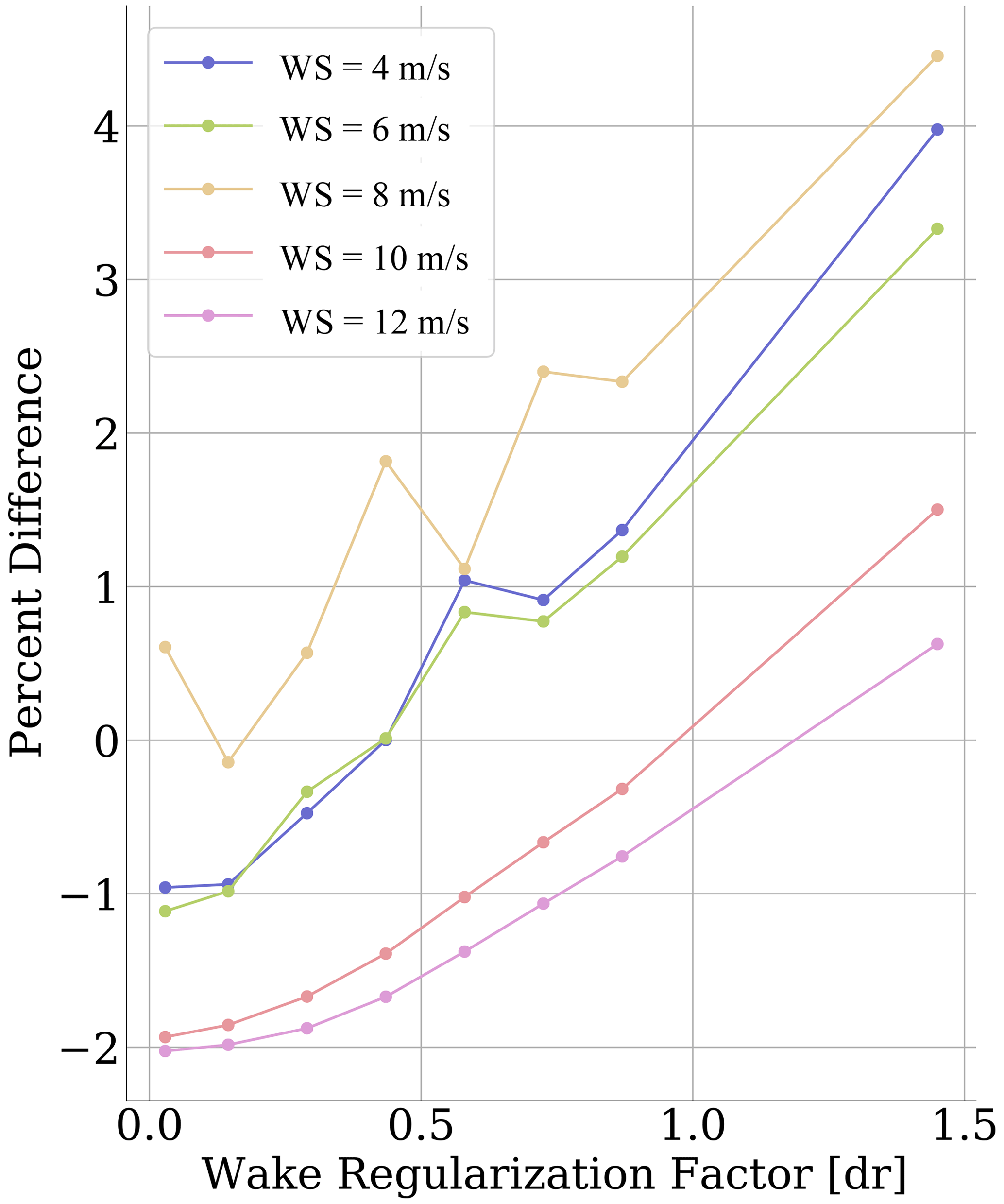
Figure 4Power percent difference between OLAF and SOWFA simulation results for various wake regularization factors. Each line color represents a different hub-height wind speed.
Table 5Recommended values selected from the results of the regularization convergence study.
In this work, the OpenFAST FVW code was compared to traditional OpenFAST BEM and actuator-line large-eddy simulation results. Comparison of the FVW method to the traditional BEM method in OpenFAST is performed using the BAR-DRC turbine used in the above studies. Large-eddy simulations were performed using the Simulator fOr Wind Farm Applications (SOWFA) (Churchfield et al., 2012). For all simulations, structural modeling was done using the structural module ElastoDyn from OpenFAST. The turbine controller was not used, and all simulations were performed at a set rotor speed and blade pitch. The tower shadow model for the blade induction and blade loads are the same for BEM and OLAF, the details of which can be found in OpenFAST (2021a). An additional tower potential flow model was used in OLAF simulations to model the effect of the tower on the wake. BEM simulations were modeled with all relevant and available BEM corrections within OpenFAST. In particular, these are the Pitt–Peters skew model, Prandtl tip- and hub-loss models, and the Minnema–Pierce dynamic stall model. Details of these models are available at Moriarty and Hansen (2005) and OpenFAST (2021a).
Table 6Variation in inflow conditions for code comparisons. All simulations were performed for a mean inflow velocity of 8 m s−1.
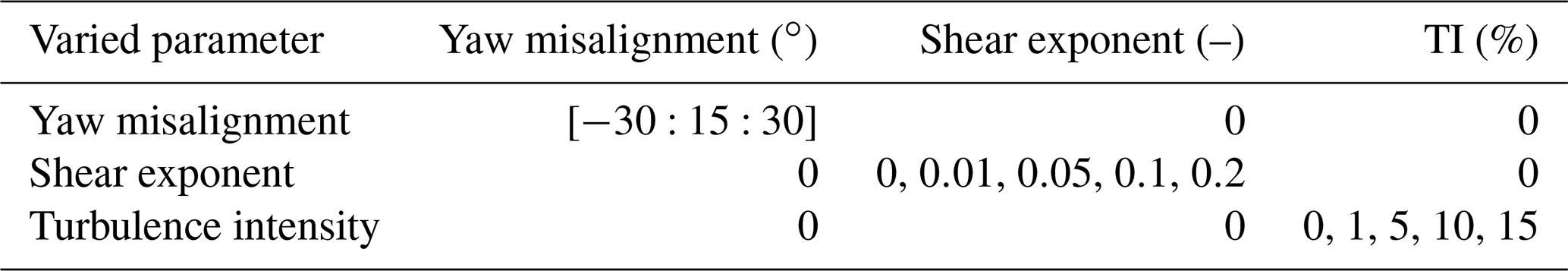
Simulations were performed at a mean hub-height inflow velocity of 8 m s−1 for a range of yaw misalignment angles, shear exponents, and turbulence intensities, as summarized in Table 6. Each parameter was varied separately, with the nominal conditions being no yaw misalignment with steady uniform inflow. For steady OpenFAST simulations, InflowWind was used to specify the hub-height inflow velocity and shear exponent. SOWFA used uniform velocity as the inflow boundary condition. For the turbulent OpenFAST simulations, ambient wind inflow was generated synthetically by TurbSim (Jonkman, 2014), which creates two-dimensional (2D) turbulent flow fields. Turbulence was simulated using the Kaimal spectrum with exponential coherence model using the standard International Electrotechnical Commission (IEC) turbulence model. The time-dependent 2D wind field was propagated along the wind direction at the mean wind speed of the midpoint of the field. Each turbulent case was simulated in TurbSim and OpenFAST six times, using six different random turbulence seeds to generate the wind data at the spatially coherent points. This was done to capture variability in the numerical simulation results associated with the uncertainty imposed by the unmeasured wind inflow. The turbulent inflow was identical for the BEM and OLAF simulations, as they are both run as part of OpenFAST and thus used the same TurbSim-generated inflow. SOWFA simulations were not conducted for turbulent inflow because it would have been impossible to use the same inflow, thus leading to questionable comparison results.
For the code-to-code comparison, the results focus on verification of statistical results between OLAF, BEM, and SOWFA. Particular attention was paid to how the comparisons changed with varying inflow conditions. Many QoIs were considered, as summarized in Table 7. All QoIs were considered time- and azimuthal-averaged quantities. Though all these QoIs were considered, only a select few are presented for much of the analysis. To include all QoIs in the analysis, box-and-whisker plots (pandas, 2022) are included, which consider all QoIs listed in Table 3. In these plots, each box shows the median value of all results (yellow line), individual QoI values (green dots), lower- (Q1) and upper-quartile (Q3) values (box edges), maximum and minimum values excluding outliers (whiskers), and outlier points (× symbols). The whiskers extend up to . Any data points outside of this range are classified as outliers, which also coincide with individual QoI values. These ranges are computed for each box, not across all data in a given figure. Thus, a value that might be an outlier for one set of results may not be for another set, even if the boxes are shown on the same plot. All inflow conditions are for steady inflow unless stated otherwise. Yaw misalignment cases were simulated in constant uniform inflow (shear exponent of 0) and sheared and TI comparison cases were simulated with no yaw misalignment.
Table 7Quantities of interest for the comparison study (FA: fore–aft, SS: side–side, OoP: out-of-plane, IP: in-plane).
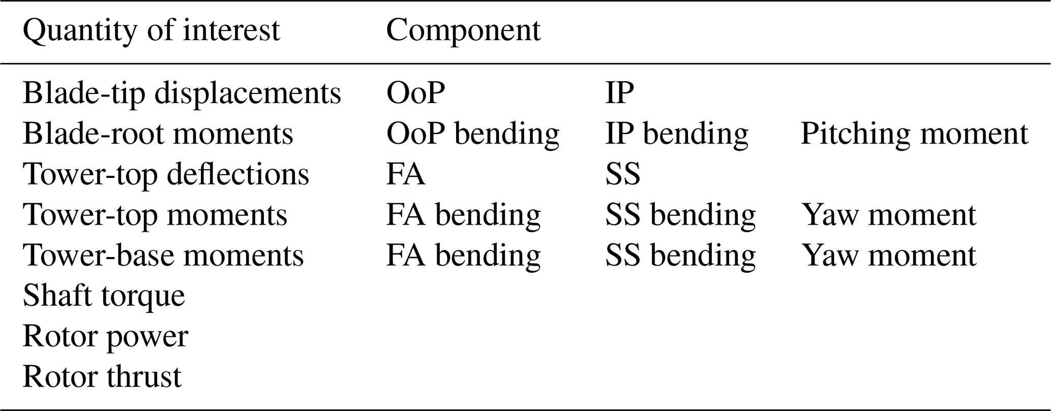
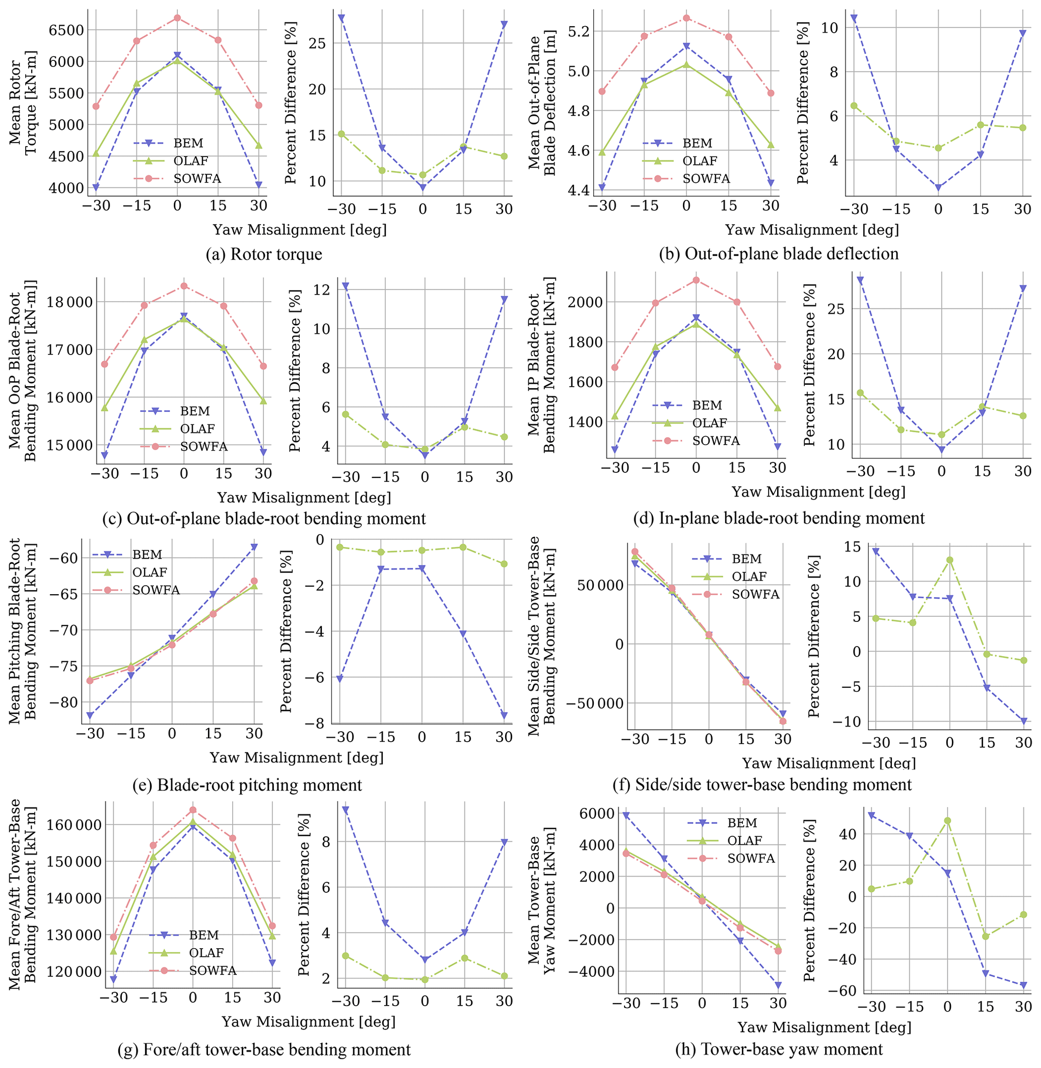
Figure 5Time-averaged quantities for OLAF, BEM, and SOWFA results with varying yaw misalignment angles. Plots on the left show mean quantities, and plots on the right show percent difference in the means from SOWFA results.
4.1 Yaw misalignment
Shown in Fig. 5 are time-averaged quantities for several QoIs from OLAF, BEM, and SOWFA simulations for a range of yaw misalignment angles, along with percent differences, computed using Eq. (5), of OLAF and BEM results relative to SOWFA results.
For all QoIs, the results from each computational method follow the same trend with changing yaw misalignment. The trend depends on the QoI, with most showing reduced values with increasing absolute yaw misalignment. Tower-base side–side and yaw moments showed decreasing values with non-absolute increasing yaw misalignment, and the blade-root pitching moment showed the opposite trend. Though the same trends were captured by each computational method, the actual results differ. In particular, OLAF and SOWFA results show comparable values with an average percent difference of < 5 % for all yaw misalignment angles, including the most extreme. However, BEM results deviated significantly more from SOWFA results for increasing absolute yaw misalignment, with percent differences at yaw misalignment of reaching up to 48.6 % for the tower-base yaw moment. Alternatively, the percent difference between OLAF and SOWFA results is < 5 % for this case, and overall results appear to be only marginally dependent on yaw misalignment. Note that the high percent difference in OLAF results for the tower-base bending moment at 0∘ yaw misalignment are artificially increased due to the small average value at this misalignment angle. Shown in Fig. 6 are box-and-whisker plots of percent difference values between the time-averaged mean and standard deviations, computed using Eq. (5), of SOWFA results and OLAF or BEM results for all QoIs listed in Table 7, except the blade distributed quantities and those with means near zero. When box-and-whisker plots are shown, each dot represents an individual QoI value (variation in x-axis location within a bar aids visualization). Box-and-whisker plots show the median (yellow line) value of all results; lower- and upper-quartile values (box edges); maximum and minimum values excluding outliers (whiskers); and outlier points (× symbols), which also coincide with individual QoI values. Percent differences in time-averaged means of BEM results increase with an increasing absolute yaw angle, averaging 5.46 % for no yaw misalignment and increasing to 15.9 % for yaw misalignment. The relative error between OLAF and SOWFA results show minimal dependence on yaw misalignment, with percent differences for all yaw misalignment angles reaching no higher than 8 %. Percent differences in standard deviation values tend to be larger for both BEM and OLAF results, averaging 20.6 % and 15.1 %, respectively, across all yaw misalignment angles. Though OLAF standard deviation values do differ with yaw misalignment, the average standard deviations across all QoIs do not seem to depend on yaw misalignment. BEM standard deviation results show dependence on yaw misalignment with increasing percent difference for large absolute yaw misalignment values but to a lesser extent than what was seen for mean values. Thus, the accuracy of BEM mean and standard deviation results compared to SOWFA results seems to decrease with increased absolute yaw misalignment, whereas OLAF accuracy stays mostly consistent regardless of yaw misalignment.
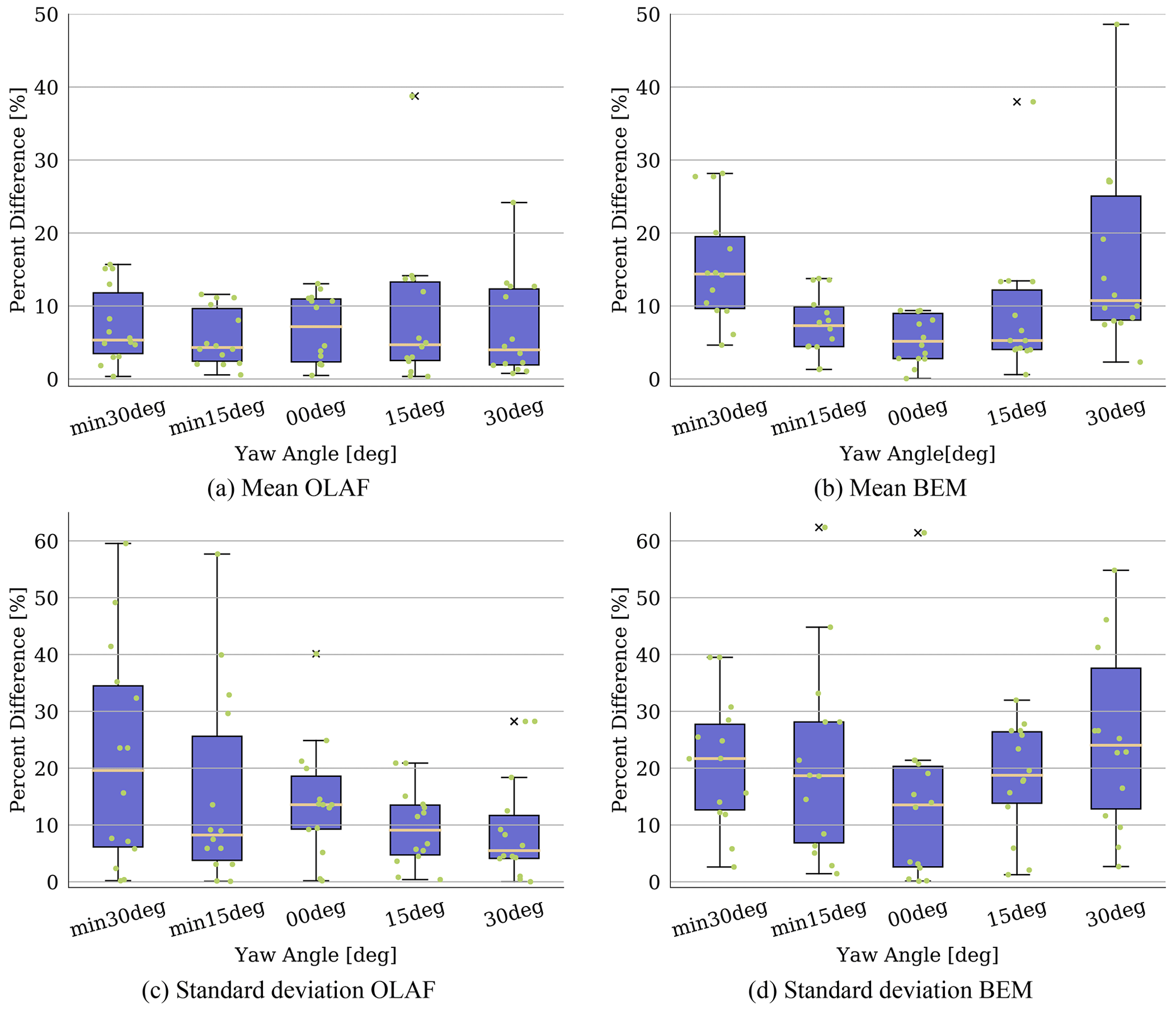
Figure 6Average percent difference between OLAF and BEM versus SOWFA results across all QoIs for varying yaw misalignment angles. Each dot represents an individual QoI value (variation in x-axis location within a bar aids visualization). Box-and-whisker plots show the median (yellow line) value of all results; lower- and upper-quartile values (box edges); maximum and minimum values excluding outliers (whiskers); and outlier points (× symbols), which also coincide with individual QoI values.
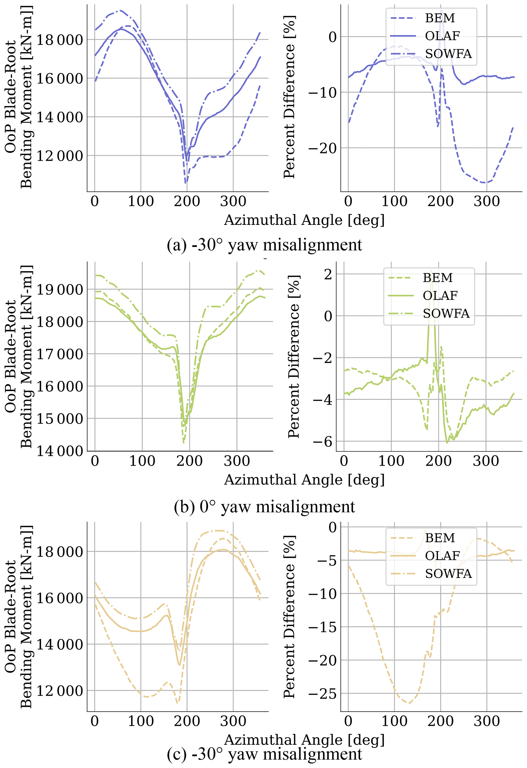
Figure 7Azimuthal-averaged quantities for OLAF, BEM, and SOWFA results with varying yaw misalignment angles. Plots on the left show mean quantities, and plots on the right show percent difference in the means from SOWFA results. Line color indicates yaw misalignment angle, and line style indicates computational method. SOWFA results are shown as a dash–dot line. OLAF results are shown as solid lines. BEM results are shown as dashed lines.
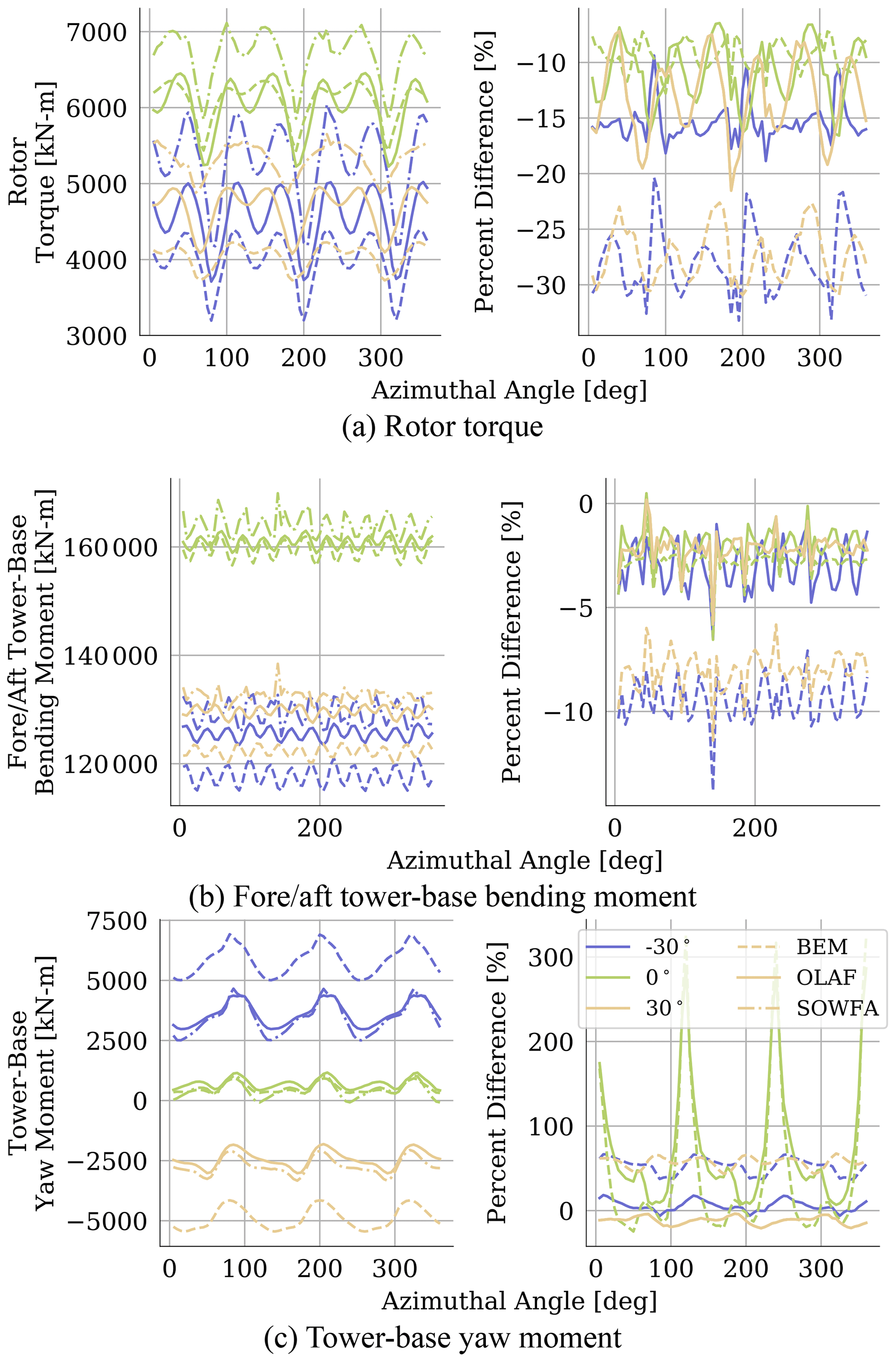
Figure 8Azimuthal-averaged quantities for OLAF, BEM, and SOWFA results with varying yaw misalignment angles. Plots on the left show mean quantities, and plots on the right show percent difference in the means from SOWFA results. Line color indicates yaw misalignment angle, and line style indicates computational method. SOWFA results are shown as a dash–dot line. OLAF results are shown as solid lines. BEM results are shown as dashed lines.
Shown in Fig. 7 are azimuthal-averaged results for the out-of-plane blade-root bending moment, with each subplot depicting a different yaw misalignment angle. Each plot shows results from all computational methods as well as percent differences in OLAF and BEM results relative to those of SOWFA. Out-of-plane blade-root bending results show a dip where the blade passes behind the tower. For these results, OLAF and SOWFA results are in close agreement for all azimuthal blade locations, though increased differences are seen behind the tower, at which point OLAF predicts a sharper drop in the bending moment. BEM results show comparable results but predict a lower bending moment at all azimuthal locations. When yaw misalignment is introduced, OLAF and SOWFA results remain comparable, again with OLAF predicting lower bending moments when passing behind the tower. As before, BEM predicts lower bending moments at all azimuthal locations, and during the portion of the blade motion where the blade is downstream of the tower, the results are actually closer to SOWFA and OLAF results. During the blade motion where the blade is not in the wake of the tower, however, BEM predicts nearly 30 % lower-bending-moment results compared to SOWFA, with performing the worst.
Shown in Fig. 8 are azimuthal-averaged results for rotor torque and tower-base fore–aft bending and yaw moments. Each plot shows results from all computational methods as well as percent differences in OLAF and BEM results relative to those of SOWFA. Note that the high percent difference at certain azimuthal angles for tower-base yaw moments is due to the SOWFA value approaching zero. For all shown QoIs, all codes follow comparable trends. Rotor torque and tower-base yaw moments show three large dips corresponding to the blade passing behind the tower. Though overall trends are comparable, clear differences are seen in BEM results at large yaw misalignment angles. For all QoIs, percent difference results for BEM and OLAF are comparably low with no yaw misalignment. However, as was seen for the mean and standard deviation results, the change at large yaw misalignment angles with BEM percent difference values are higher at all azimuthal locations. As with Fig. 6, these results clearly show that BEM accuracy varies with yaw misalignment, whereas OLAF accuracy is relatively independent.

Figure 9Computational time and average percent difference for each simulation method. Computational time is shown by the blue line corresponding to the left axis, and average percent difference is shown by the green line corresponding to the right axis. Average percent difference was computed for all results presented in this section.
While accuracy is crucial to the success of a computational method, it is important to consider the differences in computation cost of each method used in this work. Shown in Fig. 9 is a comparison between the computation time in CPU hours for each method, as well as the average percent difference values of the same quantities considered in Fig. 6. The average percent difference for SOWFA is shown as zero because this is the highest-fidelity code. Note that computational time of OLAF and SOWFA simulations is highly dependent on modeling choices, so these values will vary with setup choices. This chart clearly shows the near 2× error reduction when using OLAF instead of BEM. OLAF does, however, require significantly more computational power than BEM, with OLAF simulations taking 𝒪(40) CPU hours to complete for the simulation specifications used here, whereas BEM requires minutes. When compared to SOWFA, however, OLAF is significantly faster, with SOWFA simulations for this work requiring approximately 260 CPU hours to complete. However, OLAF and SOWFA are both parallelized codes, and so wall-clock time could be more equitable based on available resources. As always, the choice of which computational method to use is a balancing act between computational cost and accuracy. These results indicate that, given the problem being considered, OLAF could be a reasonable middle ground between engineering models and CFD.
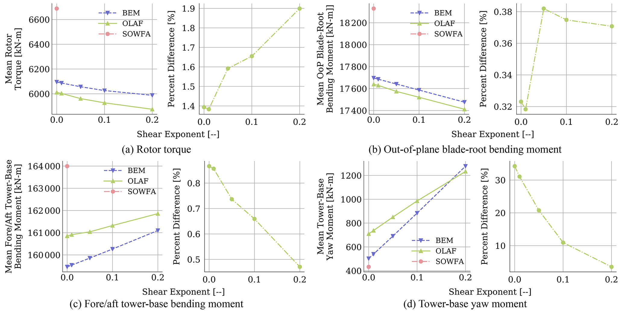
Figure 10Time-averaged quantities for OLAF, BEM, and SOWFA results with varying shear exponent. Plots on the left show mean quantities, and plots on the right show percent difference in the mean results.
4.2 Shear exponent
Shown in Fig. 10 are the time-averaged quantities for several QoIs from OLAF and BEM simulations for a range of shear exponents, along with percent differences in BEM results relative to OLAF results. Note that SOWFA results are only included here at the zero-shear point. This is because of the complexities within SOWFA of running steady inflow with a specified shear exponent as well as the additional computational expense. For all results but the tower-base yaw moment, the relative trends of OLAF and BEM are the same with changing shear exponent, though the percent difference between the results does increase slightly with increasing shear exponent. For all shear exponents, OLAF predicts higher loads for the considered components. The tower-base yaw moment, however, increases at a sharper rate for BEM results compared to OLAF results. In fact, at low shear exponents OLAF predicts a higher tower-base yaw moment, whereas BEM predicts a higher yaw moment at a shear exponent of 0.2. This results in a reduced percent difference between the methods. These results are summarized in Fig. 11, which shows box-and-whisker plots for each shear exponent, made up of the percent difference values of each QoI for the mean (left) and standard deviation (right) of the results. These results show consistent percent differences for all shear exponents across all QoIs. For mean results, percent differences increase slightly with a higher shear exponent, but median percent difference values increase by < 1 %. For standard deviation results, the median percent difference remains consistent across all shear exponents, but the upper ranges of these values do fluctuate slightly. These results indicate that though shear exponent does have a slightly higher impact on time-averaged BEM results compared to OLAF results, it is to a much lesser extent than yaw misalignment.
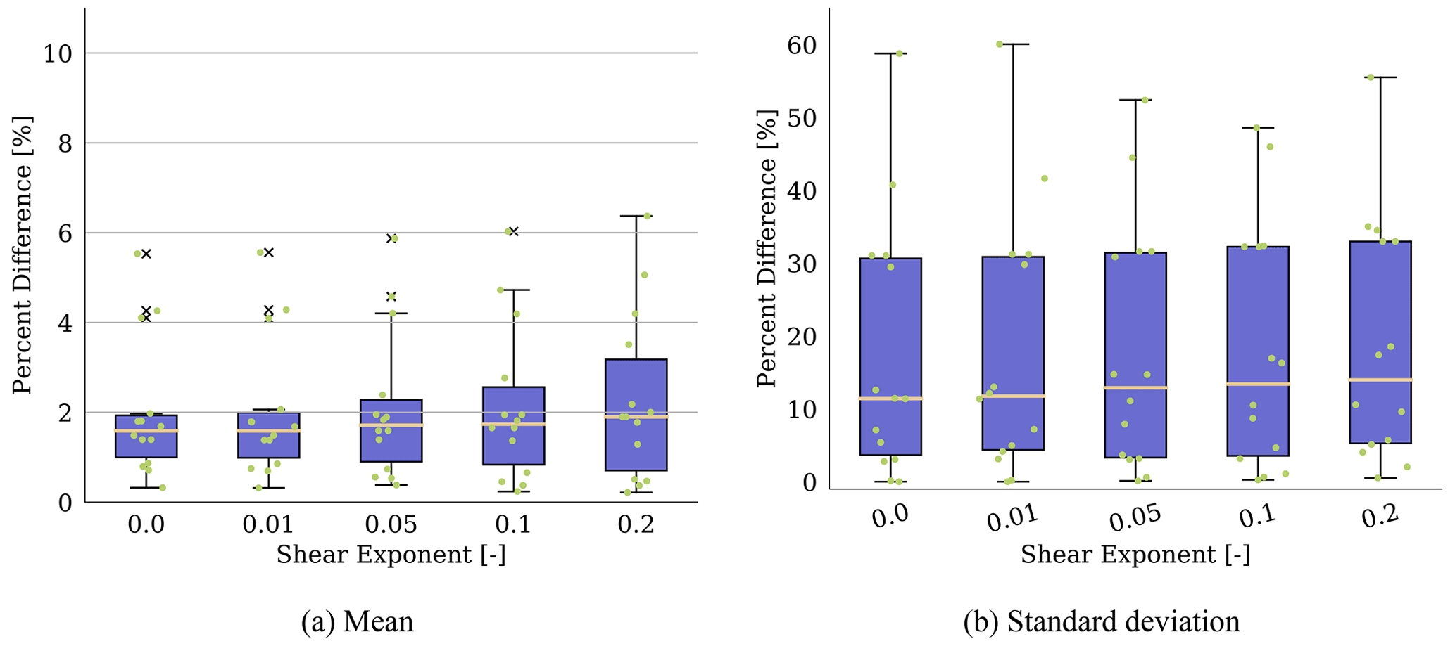
Figure 11Average percent difference between BEM and OLAF results across all QoIs for varying inflow shear exponents. Each dot represents an individual QoI value (variation in x-axis location within a bar aids visualization). Box-and-whisker plots show the median (yellow line) value of all results; lower- and upper-quartile values (box edges); maximum and minimum values excluding outliers (whiskers); and outlier points (× symbols), which also coincide with individual QoI values.
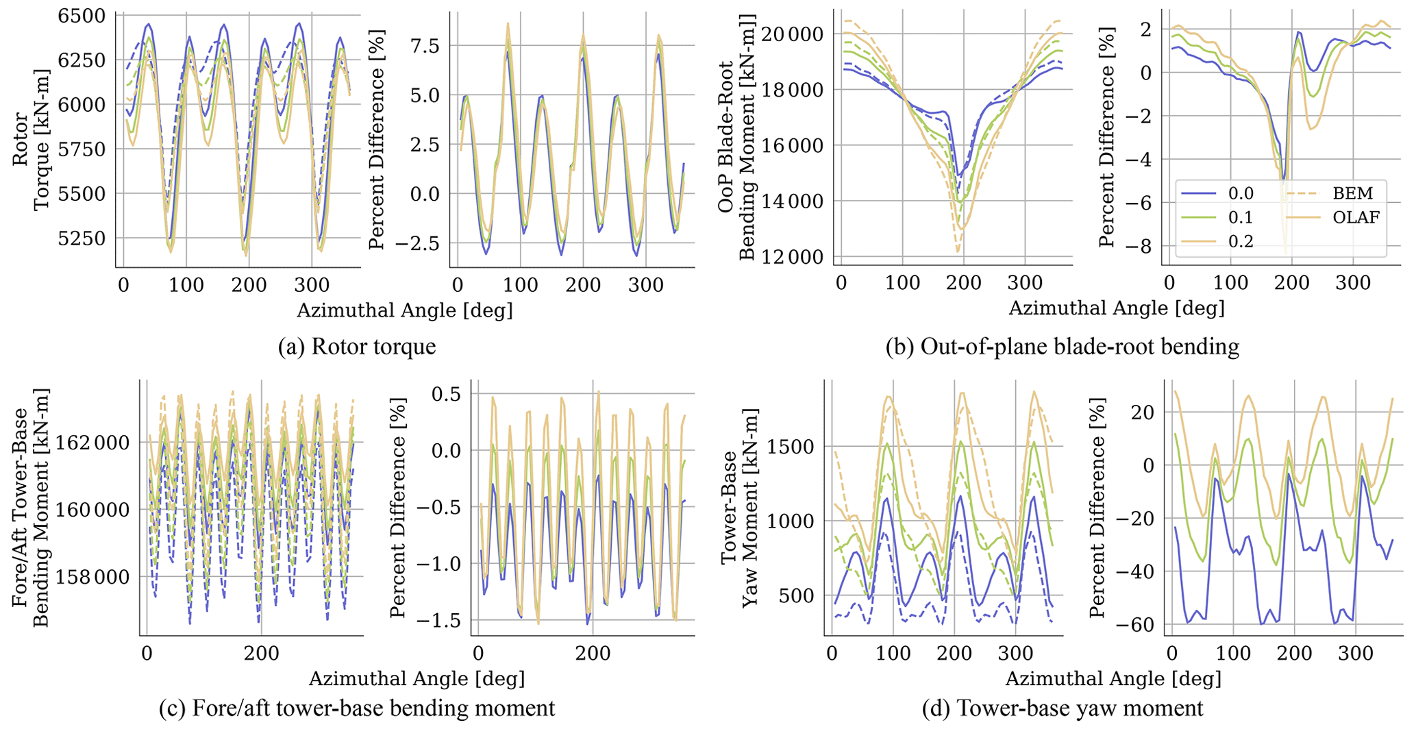
Figure 12Azimuthal-averaged quantities for OLAF and BEM results with varying shear exponent. Plots on the left show mean quantities, and plots on the right show percent difference in the means from OLAF results. Line color indicates shear exponent, and line style indicates computational method. OLAF results are shown as solid lines, and BEM results are shown as dashed lines.
Shown in Fig. 12 are azimuthal-averaged results for all computational methods, as well as percent differences between BEM and OLAF results. The overall shapes of these results are comparable to those shown for the varying yaw misalignment cases in Fig. 8. For rotor torque and tower-base fore–aft bending moment, there is a clear separation between OLAF and BEM results. For rotor torque, the results compare best at the dips corresponding to the blades passing behind the tower. For each method, there is minimal change to the results at this point in the blade path with changing shear exponent. This is expected, since the flow behind the tower is dominated by the tower wake. The flow behind the tower is also affected by the shear exponent in that the mean velocity will vary at a given height based on this value. However, based on these results, the effects are dominated by the tower wake, and shear plays a negligible role in these quantities. When the blades are not behind the tower, shear exponent has more of an effect on the results, though to a greater extent for BEM results, with a higher shear exponent resulting in reduced rotor torque. Minimal differences in the tower-base fore–aft bending moment are seen for each method. Overall, the moment increases with an increasing shear exponent, though OLAF shows an appreciably higher moment at all azimuthal angles at a shear exponent of 0.2. This results in a higher percent difference at this inflow condition. When comparing results for the out-of-plane blade-root bending moment, the largest differences are seen when the blade passes behind the tower. At this location, OLAF predicts a higher bending moment compared to BEM. For both methods, the bending moment decreases with an increasing shear exponent. The bending moment increases until the blade is above the turbine, with this maximum value increasing with an increasing shear exponent. For all shear exponents, OLAF predicts a higher bending moment than BEM. Though these overall trends are comparable between OLAF and BEM, the average percent difference between these results does increase with an increasing shear exponent, though to a greater extent when the blade is in the tower wake.
Differences in the tower-base yaw moment are considerable between OLAF and BEM, with different azimuthal trends seen at all shear exponents. For all OLAF results, the yaw moment spikes when a blade is behind the tower, followed by a sharp decrease and then another smaller spike before another blade passes behind the turbine. This trend is seen for all shear exponents, though the sharp drop becomes shallower with an increasing shear exponent. BEM results are also characterized by a spike when a blade is behind the tower. However, at low shear exponents, the value of this spike is considerably less than that predicted by OLAF and is preceded by a sharp drop to a value that remains constant until another blade passes behind the tower. This drop value is comparable to that predicted by OLAF, but the secondary bump that OLAF predicts is much reduced in the BEM results and not present at higher shear values. As the shear exponent increases, the large spike predicted by BEM surpasses that predicted by OLAF, and the sharp drop is instead a gradual reduction until the minimum value is reached. Thus, while percent difference between the methods remains large for all shear exponents, the primary takeaway is that changing the shear exponent drastically changes the azimuthal trend predicted by BEM, whereas OLAF trend changes are more subtle. While these differences are not seen for most other QoIs, it is important to note that changing the shear exponent can have a significantly different effect on azimuthal OLAF results compared to BEM results for certain important QoIs.
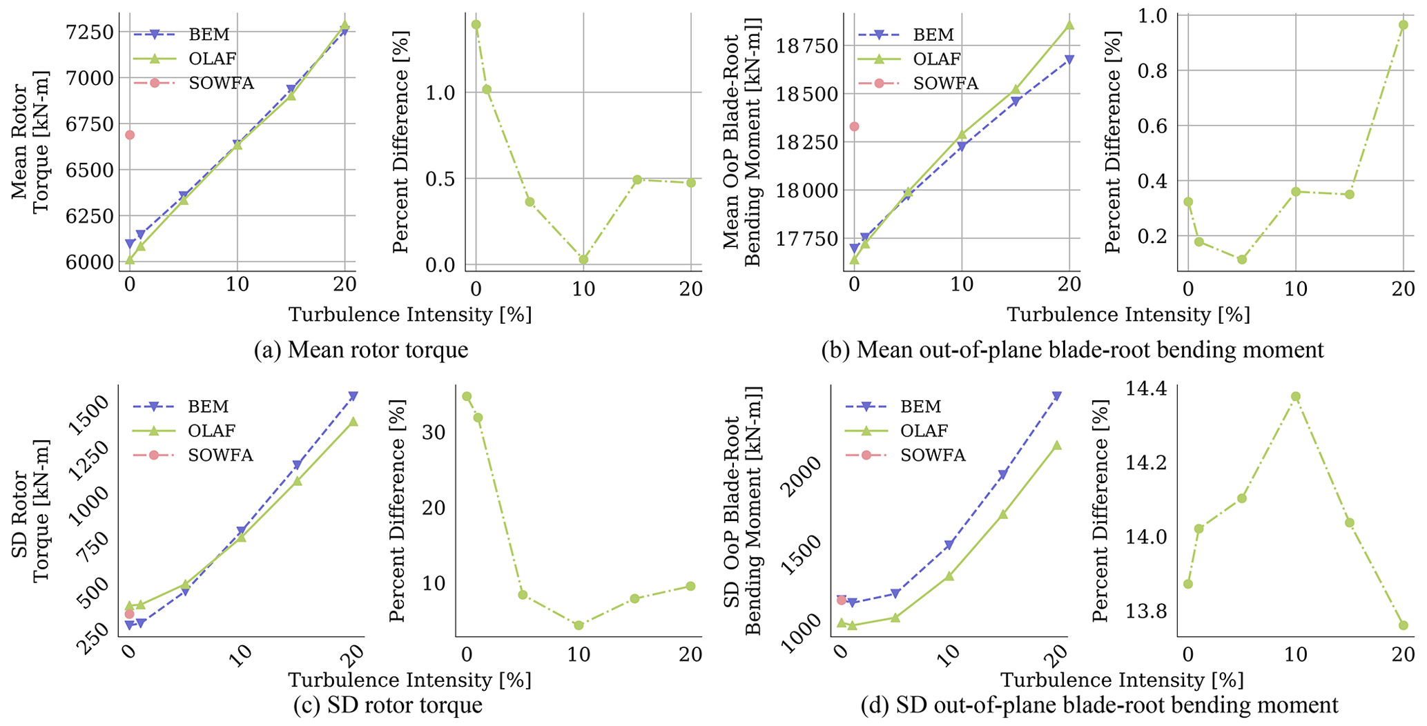
Figure 13(a, b) Time-averaged and (c, d) standard deviation quantities for OLAF, BEM, and SOWFA results with varying inflow turbulence intensity. Plots on the left show mean quantities, and plots on the right show percent difference in the means from BEM results.

Figure 14Average percent difference between BEM and OLAF results across all QoIs for varying inflow turbulence intensity levels. Each dot represents an individual QoI value (variation in x-axis location within a bar aids visualization). Box-and-whisker plots show the median (yellow line) value of all results; lower- and upper-quartile values (box edges); maximum and minimum values excluding outliers (whiskers); and outlier points (× symbols), which also coincide with individual QoI values.
4.3 Turbulence intensity
Shown in Fig. 13 are the time-averaged quantities for several QoIs from OLAF and BEM simulations for a range of TI values, along with percent differences in BEM results relative to OLAF results. In terms of mean results, varying turbulence intensity affects OLAF and BEM comparably. There is some change in percent difference for varying turbulence intensity, but it remains within a few percentage points. This is further supported in Fig. 14, which shows box-and-whisker plots for each turbulence intensity, made up of the percent difference values of each QoI for means (left) and standard deviations (right) of the results. Here, minimal differences for all QoIs are shown for mean results. However, standard deviations of results show larger changes with varying TI. Though the median percent difference value remains comparable across the TI values, the upper limit spans from 70 % for TI =0 % down to 17 % for TI ≥ 5 %. It is important to note that the output frequency for all results was 1 s, which has an effect on the computed standard deviation when turbulence intensity is included. However, as the main driver of this comparison is the relative error and the same sampling rate was used for all simulations, this is not expected to change the conclusions of this section.
Shown in Fig. 15 are azimuthal-averaged results for BEM and OLAF computational methods as well as percent differences in BEM results relative to those of OLAF. As is expected, both methods show increased variability with increasing TI. For all unsteady flow, percent difference results are comparable and there seems to be negligible change due to increasing TI. However, there is a significant change between steady and unsteady inflow. In particular, for steady flow (i.e., when TI =0 %), BEM predicts significantly larger rotor torque and out-of-plane blade-root bending moments at all azimuthal locations. However, as soon as turbulence is introduced into the inflow, this relationship flips and BEM predicts significantly lower rotor torque and out-of-plane blade-root bending moment for all azimuthal locations.

Figure 15Azimuthal-averaged quantities for OLAF and BEM results with varying inflow turbulence intensity levels. Plots on the left show mean quantities, and plots on the right show percent difference in the means from OLAF results. Line color indicates turbulence intensity level, and line style indicates computational method. OLAF result are shown as solid lines, and BEM results are shown as dashed lines.
The purpose of this work was to determine the accuracy of an aeroelastically coupled FVW method under conditions known to be challenging to lower-fidelity aerodynamic methods. This was done by comparing OLAF results to high-fidelity SOWFA results and low-fidelity BEM results for a large range of TI, shear, and yaw misalignment conditions.
Through these comparisons, it was found that for all considered QoIs, SOWFA, OLAF, and BEM results compare well for steady inflow conditions with no yaw misalignment. For OLAF results, this strong agreement was consistent for all yaw misalignment values, with percent difference values of time-averaged results remaining within 1.2 % across all QoIs and varying little with yaw misalignment. The BEM results, however, deviated significantly more from SOWFA results with increasing absolute yaw misalignment, with percent differences at a yaw misalignment of reaching up to 48.6 %. These trends were true for standard deviations of the results as well, though the BEM results showed less of a change with increasing absolute yaw misalignment.
When comparing the time-averaged OLAF and BEM results, changes to shear exponent and turbulence intensity did not have a substantial impact on the relative accuracy of the models, especially compared to the impact of yaw misalignment. An exception to this is the impact of the shear exponent on the azimuthal trends. In particular, varying the shear exponent has minimal impact on the OLAF results, whereas BEM showed more substantial changes, especially in the regions where the turbine blades are not in the tower shadow.
It must be noted that the core radius of the vortex method and actuator-line model is an important parameter that can affect the results. This study used the recommended parameters from the literature, but more research is needed to understand the effect of core radius on aeroelastic response.
Consideration must also be given to modeling computational cost. When looking at percent differences in time-averaged results for all QoIs under varying yaw misalignment, OLAF showed nearly a 2× error reduction when using OLAF instead of BEM. As with all methods, increased accuracy comes with increased computational cost, with BEM, OLAF, and SOWFA simulations taking on the order of minutes, 10 CPU hours, and 100 CPU hours to complete for the simulations performed in this work, respectively. Given the dependence of BEM results accuracy on yaw misalignment, it is likely that using the higher-accuracy FVW method is preferable for conditions of large yaw misalignment, despite the increased computational cost.
The source code for all simulation software used in this work is available for download at https://github.com/OpenFAST/openfast (OpenFAST, 2021b). Note that this is research code, and the version available here may not be the exact version used for this work. This code is developed and maintained by NREL.
Data to reproduce the figures, as well as Python scripts, are available in the following GitHub repository: https://github.com/kshaler4/OLAFValidation (last access: 25 January 2023, https://doi.org/10.5281/zenodo.7697586, Shaler et al., 2023). Interested parties may contact the authors for more information.
KS led the investigation of OLAF verification work and SOWFA and BEM comparison. BA completed the wake parameter specification studies. LAMT ran all SOWFA simulations. EB and NJ provided support for this project. KS prepared the article, with support from BA, EB, LAMT, and NJ.
The contact author has declared that none of the authors has any competing interests.
Publisher’s note: Copernicus Publications remains neutral with regard to jurisdictional claims in published maps and institutional affiliations.
The research was performed using computational resources sponsored by the U.S. Department of Energy’s Office of Energy Efficiency and Renewable Energy and located at the National Renewable Energy Laboratory.
The research has been supported by the U.S. Department of Energy, National Renewable Energy Laboratory (contract no. DE-AC36-08GO28308). Funding was provided by the Department of Energy Office of Energy Efficiency and Renewable Energy Wind Energy Technologies Office.
This paper was edited by Alessandro Croce and reviewed by Georg Raimund Pirrung and Vasilis A. Riziotis.
Ananthan, S., Leishman, J. G., and Ramasamy, M.: The Role of Filament Stretching in the Free-Vortex Modeling of Rotor Wakes, in: 58th Annual Forum and Technology Display of the American Helicopter Society International, Montreal, Canada, 2002. a
Bolinger, M., Lantz, E., Wiser, R., Hoen, B., Rand, J., and Hammond, R.: Opportunities For and Challenges to Further Reductions in the “Specific Power” Rating of Wind Turbines Installed in the United States, Wind Engineering, 45, 351–368, https://doi.org/10.1177/0309524X19901012, 2021. a
Boorsma, K., Wenz, F., Lindenburg, K., Aman, M., and Kloosterman, M.: Validation and accommodation of vortex wake codes for wind turbine design load calculations, Wind Energ. Sci., 5, 699–719, https://doi.org/10.5194/wes-5-699-2020, 2020. a
Bortolotti, P., Johnson, N., Abbas, N. J., Anderson, E., Camarena, E., and Paquette, J.: Land-based wind turbines with flexible rail-transportable blades – Part 1: Conceptual design and aeroservoelastic performance, Wind Energ. Sci., 6, 1277–1290, https://doi.org/10.5194/wes-6-1277-2021, 2021. a
Branlard, E.: Wind Turbine Aerodynamics and Vorticity-Based Methods: Fundamentals and Recent Applications, Springer International Publishing, https://doi.org/10.1007/978-3-319-55164-7, 2017. a, b
Branlard, E. and Gaunaa, M.: Cylindrical Vortex Wake Model: Right Cylinder, Wind Energy, 524, 1–15, https://doi.org/10.1002/we.1800, 2014. a
Branlard, E., Papadakis, G., Gaunaa, M., Winckelmans, G., and Larsen, T. J.: Aeroelastic Large Eddy Simulations Using Vortex Methods: Unfrozen Turbulent and Sheared Inflow, J. Phys.-Conf. Ser., 625, 1–13, https://doi.org/10.1088/1742-6596/625/1/012019, 2015. a
Churchfield, M. and Lee, S.: SOWFA | NWTC Information Portal, https://nwtc.nrel.gov/SOWFA (last access: 3 November 2021), 2021. a
Churchfield, M. J., Lee, S., Moriarty, P., Martinez, L. A., Leonardi, S., Vijayakumar, G., and Brasseur, J. G.: A Large-Eddy Simulation of Wind-Plant Aerodynamics, 50th AIAA Aerospace Sciences Meeting, AIAA, Nashville, TN, 9–12 January 2012, https://doi.org/10.2514/6.2012-537, 2012. a, b, c, d
Churchfield, M. J., Lee, S., Schmitz, S., and Wang, Z.: Modeling Wind Turbine Tower and Nacelle Effects within an Actuator Line Model, in: AIAA SciTech Forum, 33th Wind Energy Symposium, AIAA, San Diego, CA, 2 January 2015, https://doi.org/10.2514/6.2015-0214, 2015. a
Churchfield, M., Schreck, S., Martínez-Tossas, L. A., Meneveau, C., and Spalart, P. R.: An Advanced Actuator Line Method for Wind Energy Applications and Beyond, in: AIAA SciTech Forum, 35th Wind Energy Symposium, AIAA, Grapevine, TX, 9–13 January 2017, https://doi.org/10.2514/6.2017-1998, 2017. a, b
Hansen, M. O. L.: Aerodynamics of Wind Turbines, Earthscan, London, Sterling, VA, ISBN 978-1-84407-438-9, 2008. a
Hauptmann, S., Bülk, M., Schön, L., Erbslöh, S., Boorsma, K., Grasso, F., Kühn, M., and Cheng, P. W.: Comparison of the Lifting-Line Free Vortex Wake Method and the Blade-Element-Momentum Theory Regarding the Simulated Loads of Multi-MW Wind Turbines, J. Phys.-Conf. Ser., 555, 1–14, https://doi.org/10.1088/1742-6596/555/1/012050, 2014. a
Jonkman, B.: TurbSim User's Guide v2.00.00, Tech. Rep. NREL/TP-xxxx-xxxxx, National Renewable Energy Laboratory, Golden, CO, https://www.nrel.gov/wind/nwtc/assets/downloads/TurbSim/TurbSim_v2.00.pdf (last access: 3 November 2021), 2014. a
Leishman, J. G., Bhagwat, M. J., and Bagai, A.: Free-Vortex Filament Methods for the Analysis of Helicopter Rotor Wakes, J. Aircraft, 39, 759–775, https://doi.org/10.2514/2.3022, 2002. a, b, c, d
Li, A., Gaunaa, M., Pirrung, G. R., and Horcas, S. G.: A computationally efficient engineering aerodynamic model for non-planar wind turbine rotors, Wind Energ. Sci., 7, 75–104, https://doi.org/10.5194/wes-7-75-2022, 2022a. a
Li, A., Pirrung, G. R., Gaunaa, M., Madsen, H. A., and Horcas, S. G.: A computationally efficient engineering aerodynamic model for swept wind turbine blades, Wind Energ. Sci., 7, 129–160, https://doi.org/10.5194/wes-7-129-2022, 2022b. a
Martínez-Tossas, L. A., Churchfield, M. J., and Leonardi, S.: Large Eddy Simulations of the Flow Past Wind Turbines: Actuator Line and Disk Modeling, Wind Energy, 18, 1047–1060, https://doi.org/10.1002/we.1747, 2015. a, b, c
Martínez-Tossas, L. A. and Meneveau, C.: Filtered Lifting Line Theory and Application to the Actuator Line Model, J. Fluid Mech., 863, 269–292, https://doi.org/10.1017/jfm.2018.994, 2019. a
Martinez-Tossas, L. A., Churchfield, M. J., and Meneveau, C.: Optimal Smoothing Length Scale for Actuator Line Models of Wind Turbine Blades Based on Gaussian Body Force Distribution, Wind Energy, 20, 1083–1096, https://doi.org/10.1002/we.2081, 2017. a
Martínez-Tossas, L. A., Churchfield, M. J., Yilmaz, A. E., Sarlak, H., Johnson, P. L., Sørensen, J. N., Meyers, J., and Meneveau, C.: Comparison of Four Large-Eddy Simulation Research Codes and Effects of Model Coefficient and Inflow Turbulence in Actuator-Line-Based Wind Turbine Modeling, J. Renew. Sustain. Ener., 10, 1–15, https://doi.org/10.1063/1.5004710, 2018. a, b
Meyer Forsting, A. R., Pirrung, G. R., and Ramos-García, N.: A vortex-based tip/smearing correction for the actuator line, Wind Energ. Sci., 4, 369–383, https://doi.org/10.5194/wes-4-369-2019, 2019. a, b
Moriarty, P. and Hansen, A. C.: AeroDyn Theory Manual, Tech. Rep. NREL/TP-500-36881, National Renewable Energy Laboratory, Golden, CO, 2005. a
OpenFAST: AeroDyn Users Guide and Theory Manual, https://openfast.readthedocs.io/en/main/source/user/aerodyn/index.html (last access: 3 November 2021), 2021a. a, b
OpenFAST: openfast, GitHub [code], https://github.com/OpenFAST/openfast, last access: 3 November 2021b. a
pandas: Pandas DataFrame Boxplot Documentation: https://pandas.pydata.org/pandas-docs/stable/reference/api/pandas.DataFrame.boxplot.html (last access: 3 November 2021), 2022. a
Papadakis, G.: Development of a Hybrid Compressible Vortex Particle Method and Application to External Problems Including Helicopter Flows, PhD thesis, National Technical University of Athens, https://doi.org/10.13140/RG.2.2.26480.92168, 2014. a
Perez-Becker, S., Papi, F., Saverin, J., Marten, D., Bianchini, A., and Paschereit, C. O.: Is the Blade Element Momentum theory overestimating wind turbine loads? – An aeroelastic comparison between OpenFAST's AeroDyn and QBlade's Lifting-Line Free Vortex Wake method, Wind Energ. Sci., 5, 721–743, https://doi.org/10.5194/wes-5-721-2020, 2020. a
Rosenhead, L.: The Formation of Vortices from a Surface of Discontinuity, P. R. Soc. Lond. A-Conta., 134, 170–192, https://doi.org/10.1098/rspa.1931.0189, 1931. a
Shaler, K.: Wake Interaction Modeling Using A Parallelized Free Vortex Wake Model, PhD thesis, Ohio State University, Columbus, OH, https://etd.ohiolink.edu/apexprod/rws_etd/send_file/send?accession=osu1589917809170463&disposition=inline (last access: 3 November 2021), 2020. a
Shaler, K., Branlard, E., and Platt, A.: OLAF User's Guide and Theory Manual, Tech. Rep. NREL/TP-5000-75959, National Renewable Energy Laboratory, Golden, CO, https://www.nrel.gov/docs/fy20osti/75959.pdf (last access: 3 November 2021), 2020. a, b
Shaler, K., Branlard, E., and Platt, A.: OLAF User’s Guide and Theory Manual (Free Vortex Wake in AeroDyn15): https://openfast.readthedocs.io/en/main/source/user/aerodyn-olaf/index.html (last access: 3 November 2021), 2022. a, b
Shaler, K., Anderson, B., and Martinez-Tossas, L. T.: Dataset for Comparison of OLAF, BEM, and SOWFA Turbine Response, Zenodo [data set], https://doi.org/10.5281/zenodo.7697586, 2023. a
Sørensen, J. N. and Shen, W. Z.: Numerical Modeling of Wind Turbine Wakes, J. Fluid. Eng., 124, 393–399, https://doi.org/10.1115/1.1471361, 2002. a, b
van Garrel, A.: Development of a Wind Turbine Aerodynamics Simulation Module, Tech. Rep. ECN-C–03-079, ECN, https://repository.tno.nl/islandora/object/uuid:869176a8-9d36-4806-94b4-aa2307aefade (last access: 3 November 2021), 2003. a, b
Vatistas, G. H., Koezel, V., and Mih, W. C.: A Simpler Model for Concentrated Vortices, Exp. Fluids, 11, 73–76, https://doi.org/10.1007/BF00198434, 1991. a
Voutsinas, S. G.: Vortex Methods in Aeronautics: How to Make Things Work, Int. J. Comput. Fluid D., 20, 3–18, https://doi.org/10.1080/10618560600566059, 2006. a
Weller, H. G., Tabor, G., Jasak, H., and Fureby, C.: A Tensorial Approach to Computational Continuum Mechanics Using Object-Oriented Techniques, Comput. Phys., 12, 620–631, https://doi.org/10.1063/1.168744, 1998. a
Winckelmans, G. S. and Leonard, A.: Contributions to Vortex Particle Methods for the Computation of Three-Dimensional Incompressible Unsteady Flows, J. Comput. Phys., 109, 247–273, https://doi.org/10.1006/jcph.1993.1216, 1993. a