Computational fluid dynamics (CFD) modeling of actual eroded wind turbine blades

Leading edge erosion (LEE) is one of the most critical degradation mechanisms that occur with wind turbine blades (WTBs), generally starting from the tip section of the blade. A detailed understanding of the LEE process and the impact on aerodynamic performance due to the damaged leading edge (LE) is required to select the most appropriate leading edge protection (LEP) system and optimize blade maintenance. Providing accurate modeling tools is therefore essential.

This paper presents a two-part study investigating computational fluid dynamics (CFD) modeling approaches for different orders of magnitudes in erosion damage. The first part details the flow transition modeling for eroded surfaces with roughness on the order of 0.1–0.2 mm, while the second part focuses on a novel study modeling high-resolution scanned LE surfaces from an actual blade with LEE damage on the order of 10–20 mm (approx. 1 % chord); 2D and 3D surface-resolved Reynolds-averaged Navier–Stokes (RANS) CFD models have been applied to investigate wind turbine blade sections in the Reynolds number (Re) range of 3–6 million.

From the first part, the calibrated CFD model for modeling flow transition accounting for roughness shows good agreement of the aerodynamic forces for airfoils with leading-edge roughness heights on the order of 140–200 µm while showing poor agreement for smaller roughness heights on the order of 100 µm. Results from the second part of the study indicate that up to a 3.3 % reduction in annual energy production (AEP) can be expected when the LE shape is degraded by 0.8 % of the chord, based on the NREL5MW turbine. The results also suggest that under fully turbulent conditions, the degree of eroded LE shapes studied in this work show the minimal effect on the aerodynamic performances, which results in a negligible difference to AEP.

1 Introduction

Leading edge erosion (LEE) is one of the most critical degradation mechanisms that occur with wind turbine blades (WTBs), generally starting from the tip section of the blade. The tip section, due to higher speeds, contributes to the majority of the torque production. The last 15 % of the blade radius for a multi-megawatt rotor can contribute up to 25 % of the total power production and more than 5 % reduction of annual energy production (AEP) for a wind farm. Eroded blades result in sub-optimal rotor performance and a significant loss of AEP of the wind turbine. In addition, the influence of surface roughness in the form of light erosion or contamination is of great practical importance for many flow applications and of particular interest to the wind industry. This form of the blade degradation process is known to accelerate the boundary layer transition to result in substantial loss of the blade's aerodynamic performance (Sareen et al., 2014).

The higher flow speeds at the blade tip also result in a higher impact velocity of the rain droplets on the blade surface, which shortens the incubation time and increases the erosion damage rate on the leading edge (LE) of the blade. A detailed understanding of the LEE process and the impact on aerodynamic performance due to the damaged LE is required to select the most appropriate leading edge protection (LEP) system and to optimize blade maintenance. Providing accurate modeling tools is therefore essential.

This paper presents a two-part investigation in which the first part focuses on accurate prediction tools for simulating various roughness distributions (on the order of 0.1–0.2 mm) due to light erosion or contamination and its influence on boundary layer transition. Roughness is a texture of the surface different from the ideal flat surface. The roughness can be both regress into the surface such caused by wear and above the surface for instance by deposits and contamination. However, erosion damage has a specific local effect on the surface morphology caused by wear to vary in shape and depth under the surface.

The erosion impact studied in the first part is assumed to be uniformly distributed at the minimal scales, where the effect of roughness is on the same order of magnitude. Larger scales of erosion where a significant amount of material is lost cannot be assessed the same way; instead, it can be thought of as a negative imprint of roughness at larger scales, which requires the explicit modeling of the actual surfaces. The second part will focus on exactly that and demonstrates the explicit modeling of high-resolution scanned LE surfaces from an actual blade with LEE damage on the order of 10–20 mm.

The novel aspect of this work is the modeling of high-resolution LE surfaces of an actual blade with LEE damage, which was captured in the field using state-of-art optical 3D scanning technologies. This makes this study different from numerically assumed damaged blades with generalized damage profiles on the LE. Previous studies (Forsting et al., 2022; Veraart, 2017; Ortolani et al., 2022) have shown an extensive effort on 2D computational fluid dynamics (CFD) studies using scaled LEE geometry based on scanned or numerically assumed geometry. Some of these works (Forsting et al., 2022; Veraart, 2017) were studied using scaled erosion profiles from a whirling arm rain erosion test, while in this work we demonstrate 3D CFD modeling of raw LE surfaces scanned from an actual blade with LEE damage. This method allows for a quantitative assessment of the effect of actual damage on the performance. Secondly, the scanning method offers the possibility to monitor damage to the blade with inspections, which has added value for an operator in choosing the right O&M and control strategy for the wind turbine.

Using the point cloud data, 2D and 3D Reynolds-averaged Navier–Stokes (RANS) CFD models have been applied to investigate the influence of shape change at the LE on aerodynamic performance. Both models are shown to predict the change in flow characteristics due to the LE differences. The simulations indicated that depending on erosion conditions the lift and drag coefficients can be reduced and increased, respectively. The results from CFD simulation have been used in a blade element momentum (BEM) model to calculate and establish the performance of the WTBs in terms of power coefficient and relative changes in AEP for both clean and eroded cases.

The following section will detail Part 1 of the paper, which focuses on the transition modeling for rough surfaces. Firstly it will briefly introduce the modeling approach and the objective of the study, and then the simulation setup is described. Then an extensive effort to study the baseline transition model is detailed with validation results for flat plate and airfoil geometries. Hereafter, the numerical detail of modeling roughness with transition is presented, which is then calibrated with experimental measurements and a discussion on the result is presented subsequently.

Thereafter, the work on Part 2 of the paper is presented. This section is a follow-up to Part 1. This section will apply CFD models discussed in Part 1 to an actual scanned geometry of eroded LE. Initially, the objective of this part of the study is presented, and then the background information on the field measurement campaign with the details on laser scanning technology is given. Then, the details on the translation of the measured geometry to CFD are presented with results on modeling 3D scanned surfaces. Thereafter, a study evaluating the sensitivity of different levels of erosion based on the scanned geometry is presented with the corresponding impact on AEP, and at the end, a discussion is presented on the results from Part 2.

Finally, the conclusion is presented based on the results from this two-part study.

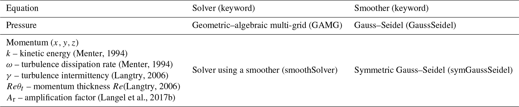
(Menter, 1994)(Menter, 1994)(Langtry, 2006)(Langtry, 2006)(Langel et al., 2017b)

Table 1 The flow equations and the corresponding solvers used within OpenFOAM.

2 CFD transition model for rough surfaces (Part 1)

The boundary layer transition process is an extremely complicated process that has been studied extensively for almost a century. During this phenomenon, the flow characteristics are changed from a streamlined laminar flow to a chaotic turbulent flow. Modeling flow transition for wind turbine blades has previously shown promising results for validating computational models (Vimalakanthan, 2014). Accurate prediction tools for simulating various roughness distributions and their influence on boundary layer transition are therefore fundamental for efficient design optimization and implementation of wind power systems.

Turbulent modeling in general is one of the important steps taken to achieve a credible CFD solution. A closed-form solution to the turbulent Navier–Stokes equations does not exist, and computing directly for all scales is computationally expensive. Therefore Reynolds decomposition (RANS) is applied to model the turbulence with a finite degree of freedom. An eddy viscosity model using the Boussinesq hypothesis is used to resolve the Reynolds stresses and fluxes, which models only the isotropic turbulence.

Many years of research and development have delivered numerous turbulence models to resolve this isotropic turbulent flow field. However, due to its robust prediction of the onset and the level of flow separation under adverse pressure gradients, Menter’s k−ω shear stress transport (SST) model (Menter, 1994) has been extensively adopted for external aerodynamics and high Re simulations. About a decade later from his publication on the SST model, Menter with Langtry (2006) formulated the γ−Reθ_t correlation-based SST model (SSTLM) for adding the effect of laminar–turbulent flow transition. This part of the paper will demonstrate the development of incorporating yet another effect of distributed roughness into the SSTLM turbulence model.

The objective of this part of the study was to develop and calibrate the roughness amplification model for SSTLM model within the open-source flow solver OpenFOAM (Jasak et al., 2007). This model was originally envisaged by Dassler, Kozulovic, and Fiala (Dassler et al., 2010, 2012) in 2010, and recently in 2017 Langel et al. (2017b) from Sandia National Laboratory published a detailed thesis on this model implementation into the flow solver OVERFLOW-2. The work of Langel et al. (2017b) was used as the basis for this development and calibration of the roughness amplification model for OpenFOAM.

This model implementation allows for 2D and 3D boundary layer transitional CFD simulations including the effect of surface roughness. This is achieved via an additional transport equation for modeling roughness onto a pre-existing transition model. This approach uses an additional field variable, the roughness amplification quantity (A_r) to be transported downstream to generate a region of influence due to the prescribed roughness; thus the underlying transition model is triggered accounting for the effect of surface roughness.

Firstly, the results from validating the underlying transition model within the OpenFOAM solver are applied to clean surfaces. For verification purposes, the results are also compared against the panel code XFOIL. Then the implementation of the transport equation-based roughness model and its calibration study for airfoil sections with rough LE are presented accordingly.

Figure 1 Computed residuals for NACA 63-418 with rough LE with 200 µm roughness height at $\mathrm{AoA}=\mathrm{4}{}^{\circ }$.

2.1 Simulation setup – OpenFOAM

The steady-state incompressible simpleFoam solver was used for all OpenFOAM simulations. The name comes from the fact that simpleFoam uses the Semi-Implicit Method for Pressure-Linked Equations (SIMPLE) algorithm of Patankar and Spalding to enforce the pressure/velocity coupling. It is a steady-state solver for incompressible turbulent flows. It can be used with a variety of turbulence models which are available in OpenFOAM. The momentum equations are solved using the second-order bounded Gauss linearUpwind scheme. The turbulence closure relations are solved using the bounded Gauss limitedLinear numerical scheme that limits towards first-order upwind in regions of rapidly changing gradient, while other parts of the domain are resolved using second-order linear scheme to achieve greater numerical stability.

The GAMG (geometric–algebraic multi-grid) solver was used for pressure equation. GAMG solver also requires a smoother for its operation; thus once again GaussSeidel smoother was used with GAMG to ensure a faster convergence. The size of the initial coarse mesh is specified through in the nCellsInCoarsestLevel entry, which was specified to be 1000 based on 24 cpu computations. The agglomeration of cells is performed by the selected FaceAreaPair method. Table 1 details the OpenFOAM solvers that were used to solve all the corresponding equations describing the system.

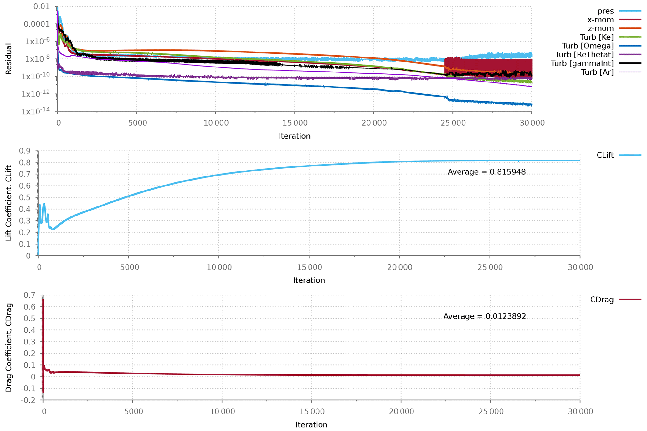
Numerical convergence was assessed based on the absolute rms residual for all equations $\mathit{<}\mathrm{1}\times {\mathrm{10}}^{-\mathrm{7}}$ or a relative reduction of 5 orders of magnitudes for all simulations with a steady hysteresis on the lift and drag forces (Fig. 1).

Figure 2 The grid and the boundary condition used to simulate the T3A test case.

Figure 3 Turbulence kinetic energy and Wall shear stress along clean flat plate.

2.2 Flow transition prediction on clean surfaces – validation/verification study

The roughness amplification model uses Langtry–Menter's local correlation-based transition model (SSTLM) (Langtry, 2006; Langtry and Menter, 2009) as the underlying model to trigger boundary layer transition, while the fully turbulent parts of the domain are resolved with Menter's k−ω SST model (Menter, 1992). In order to establish the performance of the underlying transition model, two test cases were studied to verify and validate with experimental measurements.

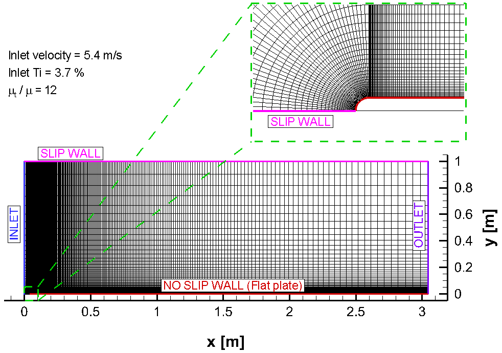
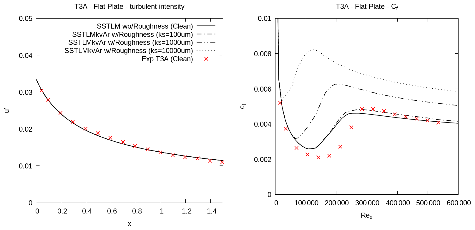
The first test case was conducted using the EROCOFTAC T3A (zero pressure gradient) experiments studying a flat plate geometry (Savill, 1993), which has become a renowned benchmark case for validating computational transition models. The simulated T3A geometry (20 mm thick flat plate with LE diameter of 15 mm) and the corresponding boundary conditions are presented in Fig. 2. Due to the inherent decay of turbulence with RANS modeling, a slightly higher turbulence intensity (3.7 %) compared to the experimented 3 % was prescribed at the inlet to match the value measured at the start of the flat plate.

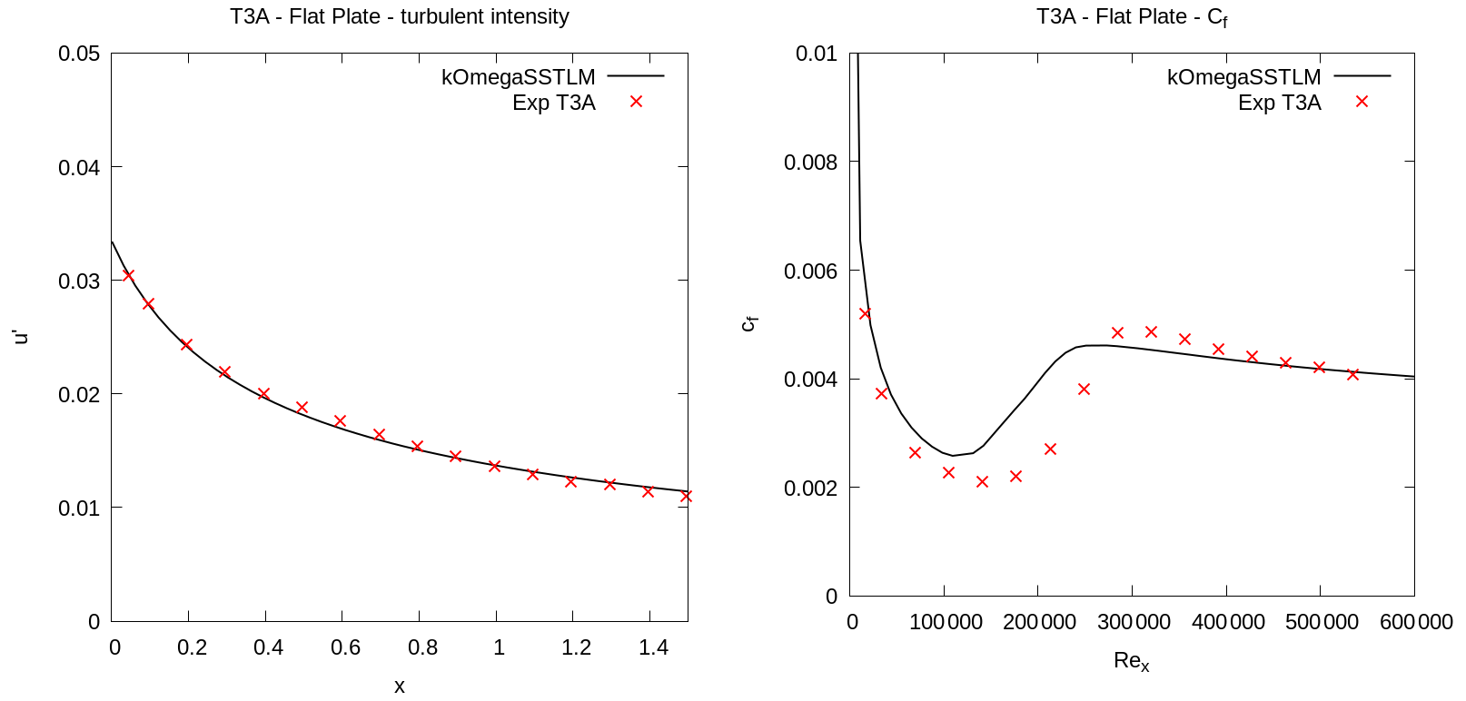
The computed turbulent kinetic energy profile and the wall shear stress along the flat plate was compared against the measurements (Fig. 3). The turbulent kinetic energy profile is defined simply as the fluctuation in streamwise velocity (u^′) to comply with experimental data set from Savill (1993), where T3A experiments have measured u^′ using hot-wire probe traverse taken 30 mm distance from the top of flat plate. Based on these results (Fig. 3) the underlying transition model (SSTLM) accurately predicts the decay of measured turbulence intensity; however, the transition point is predicted earlier than measured.

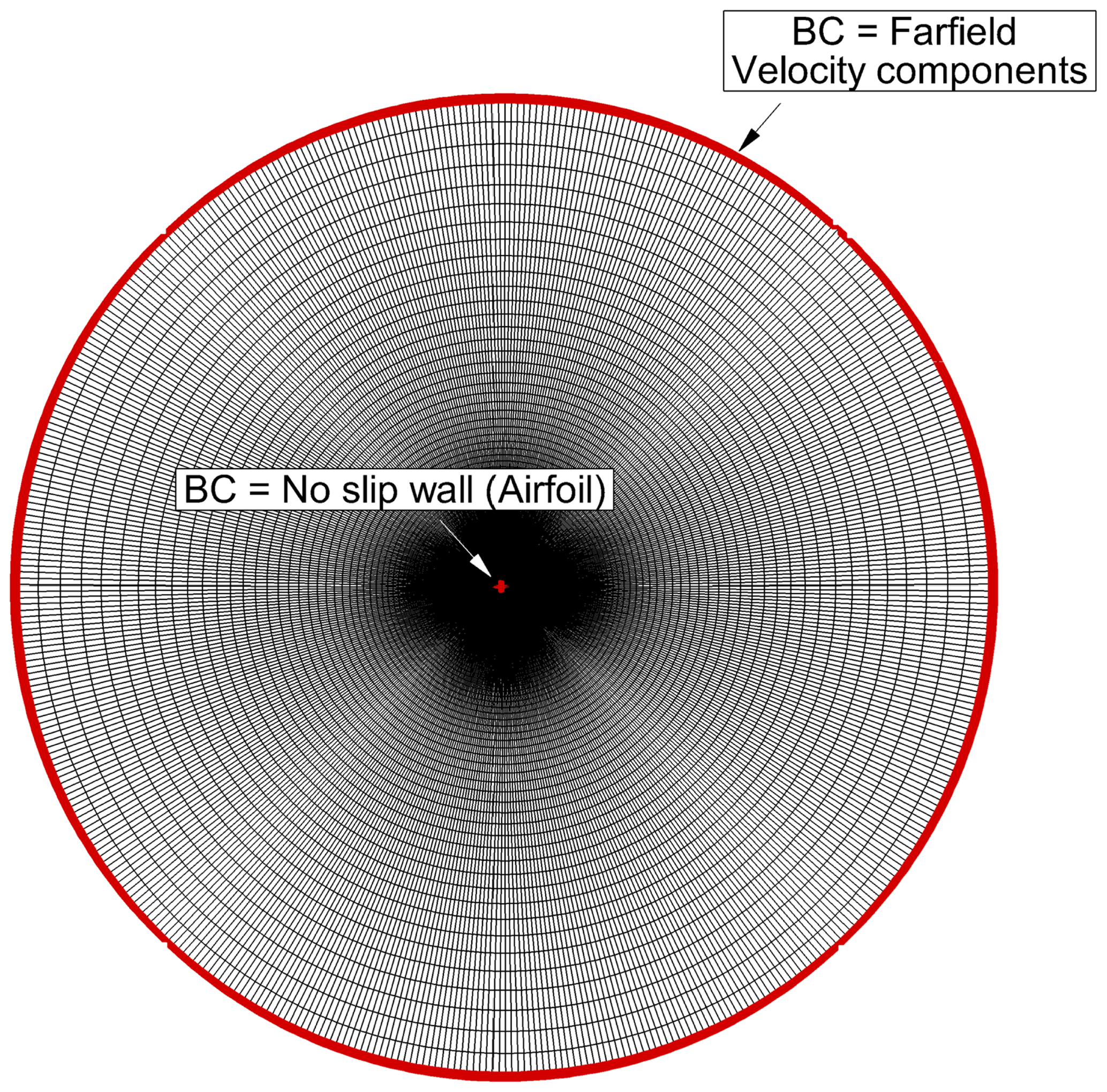
Figure 4 O-grid with 90-chord domain extent showing the full hex grid with boundary conditions.

Figure 5 Comparing results for different grid densities.

Figure 6 Comparing results for different y+ values.

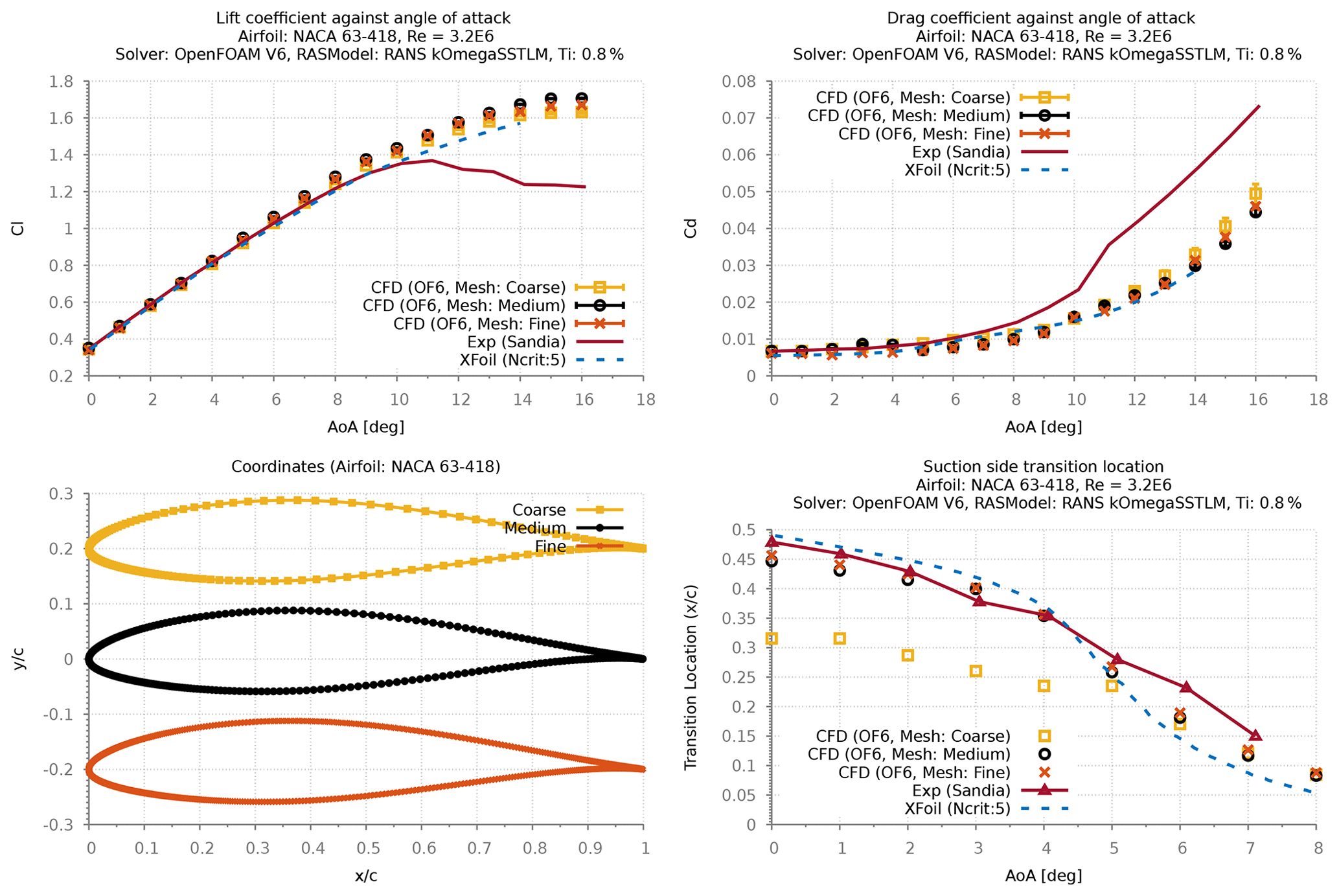
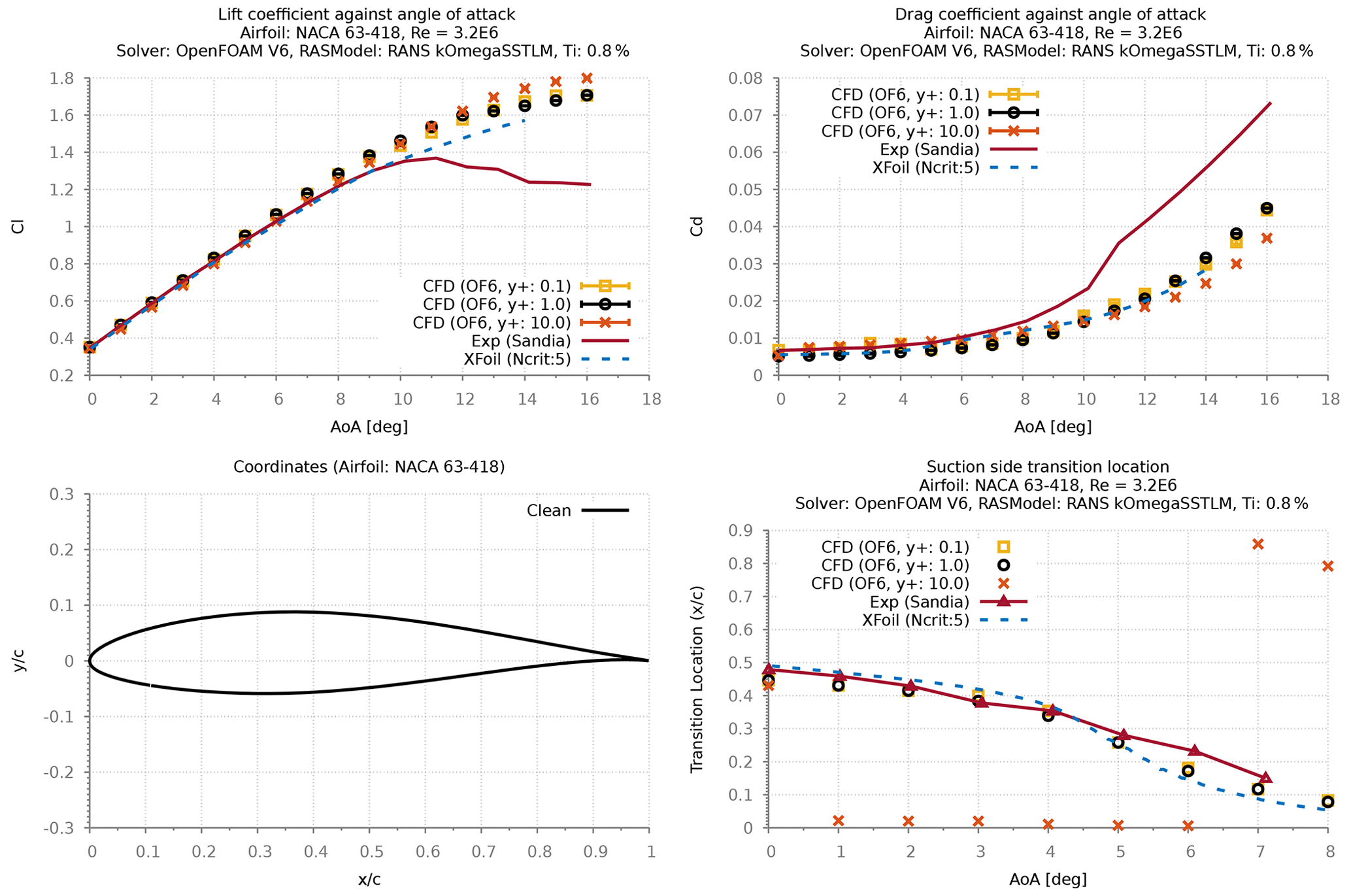
The second test case was conducted using Sandia's experimental study (LEES-Dataset) (David et al., 2020) using NACA 63-418 airfoil at three different Re (2.4×10⁶, 3.2×10⁶ and 4.0×10⁶). Based on in-house experience/sensitivity study, the 2D RANS CFD simulations were all performed with a domain extent of 90 chords (Fig. 4). The results from the grid refinement study (Fig. 5) showed that a minimum of 350 points (mesh: medium) are required to resolve the airfoil section to achieve a grid-independent solution. Similarly, a study assessing different initial grid heights normal to the wall (Fig. 6) has revealed that a minimum y+ value of 1 is required to achieve physical transitional results. The transition location was evaluated based on the rapid increase in intermittency variable (gamma), as detailed in Vimalakanthan (2014).

In the initial stages of this investigation, the original NACA 63-418 airfoil geometry from Abbott et al. (1945) was used to verify numerical accuracy as also used for a validation study by Wilcox et al. (2017). However, there has been some uncertainty about the exact geometry used in the experiment. Different publications using this experimental dataset (LEES-Dataset) for validating their numerical models have considered slightly different geometries, such as using the original geometry (Wilcox et al., 2017) defined by Abbott et al. (1945), while others have considered the geometric definition using a Bézier curve (Langel et al., 2017a).

The reason which pleads for the Bézier geometry is that in their publication, Langel et al. (2017a) have provided the control points to be able to regenerate the potential experimental geometry in a continuous fashion for numerical simulations. This Bézier curve is consistent with the interpolated model coordinates provided by Ehrmann et al. (2017) in his thesis, where he has described the experimental model coordinates being interpolated directly from the geometry of Abbott et al. (1945). The experimental pressure taps locations from the Sandia's LEES-Dataset (David et al., 2020), which is also consistent with the Bézier curve.

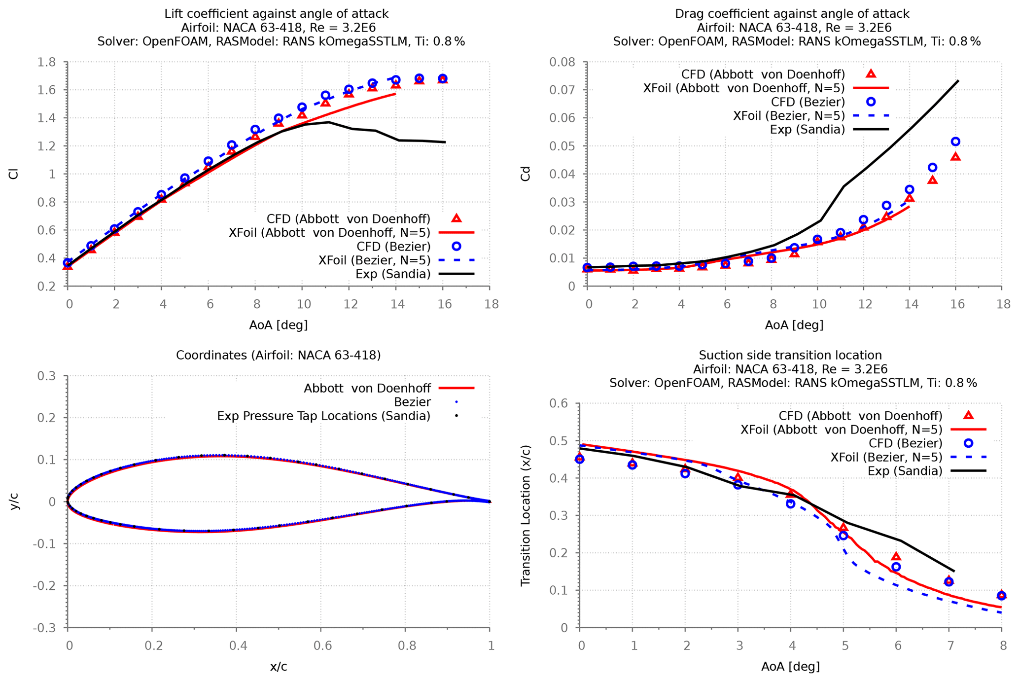
Figure 7 Comparing results for different NACA 63-418 geometries used to validate Sandia experiments.

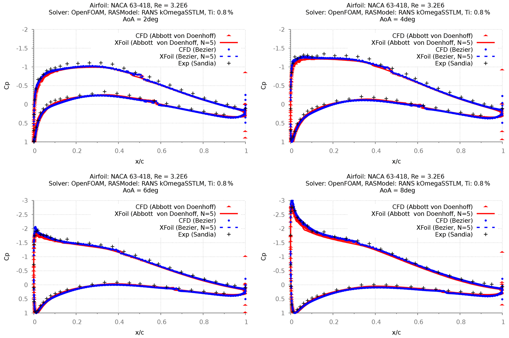
Figure 8 Comparing surface pressure distribution for different NACA 63-418 geometries used to validate Sandia experiments.

Figure 9 Validation results at $Re=\mathrm{2.4}\times {\mathrm{10}}^{\mathrm{6}}$ using the Abbott and von Doenhoff's NACA 63-418.

Figure 10 Validation results at $Re=\mathrm{4.0}\times {\mathrm{10}}^{\mathrm{6}}$ using the Abbott and von Doenhoff's NACA 63-418.

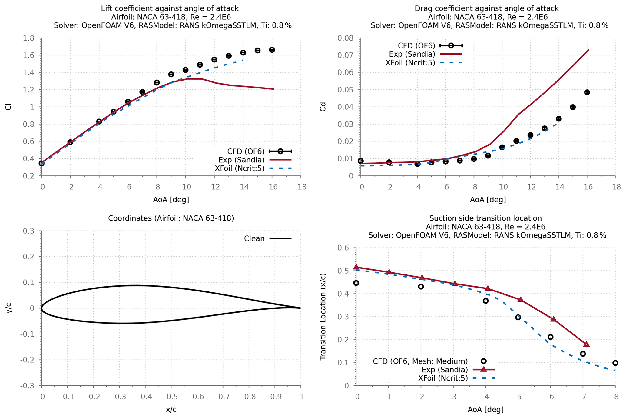
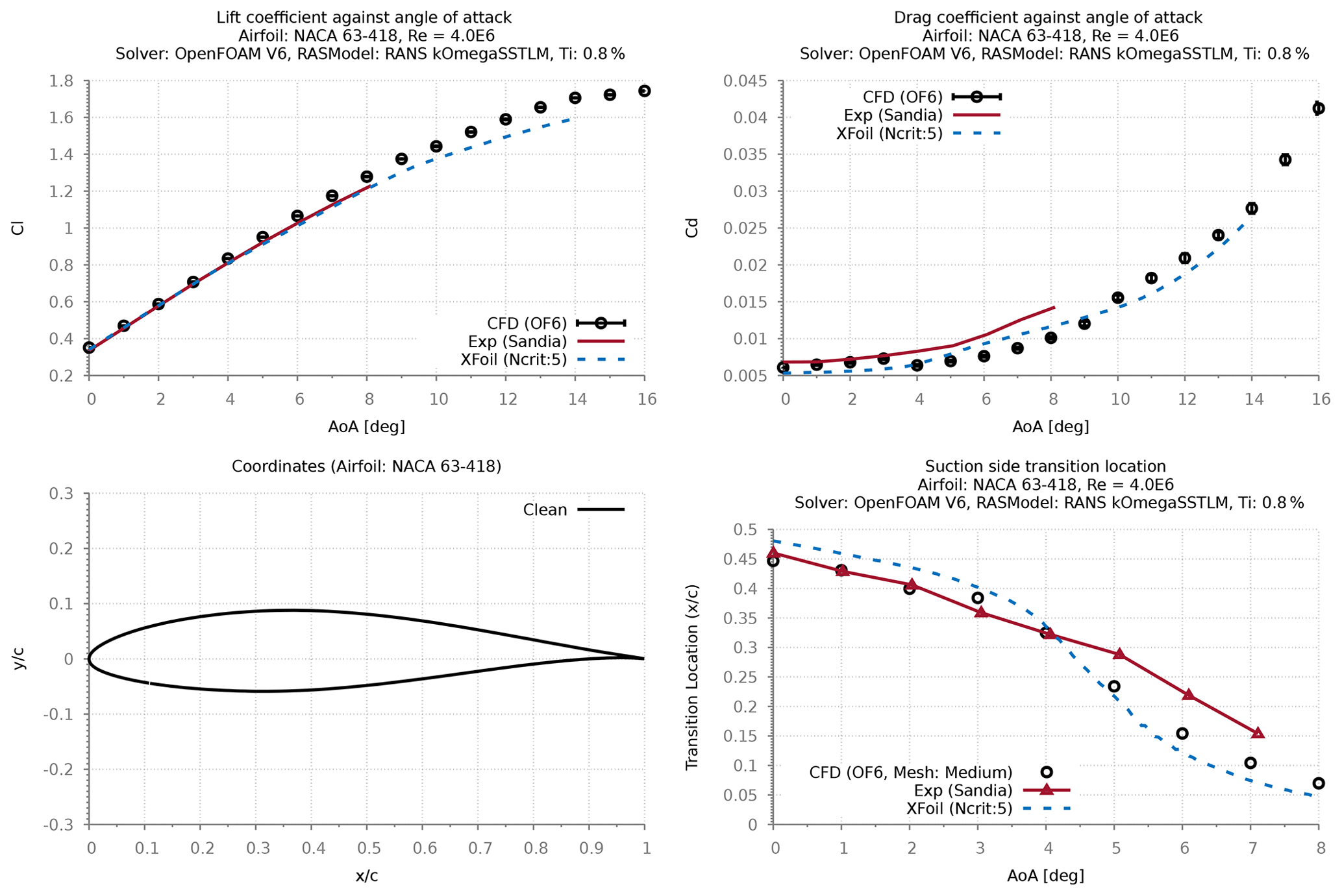
Despite having very small differences between the geometries, results comparing the numerical simulations of both geometries (Fig. 7) have revealed that better validation is achieved using the original geometry of Abbott et al. (1945), while the computed lift coefficients are slightly overpredicted with the Bézier geometry. Comparing the surface pressure distribution has shown that XFOIL and CFD results slightly under-predict the measured pressure values, irrespective of the geometry. It is noted that despite showing negligible differences between the computed pressure distributions for both geometries, for three different Re (Figs. 7–10) the validation results with the original geometry of Abbott et al. (1945) show good agreement between the calculated and measured lift curve slope.

Nevertheless, the findings from both of the aforementioned test cases make clear that the intended underlying SSTLM model is able to capture transition locations that agree well with the measurements, particularly for the Sandia experiment (David et al., 2020) using the original of Abbott et al. (1945) or the Bezier form of the NACA 63-418 geometry from Langel et al. (2017b). However, to be consistent with the original experimental work as reported in Ehrmann et al. (2017) (best measurement of the as-tested model) the Bézier geometry was chosen for calibrating the roughness amplification model.

It is also noted that this study was conducted using the SSTLM model originally implemented by Menter without the modification proposed by Langel et al. (2017b). The SSTLM model uses the relationship between the Van Driest and Blumer’s vorticity Reynolds number (Van Driest and Blumer, 1963) and the momentum thickness Reynolds number (Eq. 1) to predict separation-induced transition. In order to reduce sensitivity to free stream turbulence values, Langel et al. (2017b) have adopted the recommendation from Khayatzadeh and Nadarajah (2014) to use a different transition onset equation. This was accomplished by increasing the constant from 2.193 to 3.29 in the onset equation. However, the results from this verification study clearly show good agreement with the measured transition locations without this modification; thus the value of 2.193 originally implemented by Menter was used throughout this work.

$$\begin{array}{}\text{(1)}& R{e}_{\mathit{\nu }}={\displaystyle \frac{\mathit{\rho }{y}^{\mathrm{2}}}{\mathit{\mu }}}\left|{\displaystyle \frac{\partial u}{\partial y}}\right|;R{e}_{\mathit{\theta }}={\displaystyle \frac{max\left(R{e}_{\mathit{\nu }}\right)}{\mathrm{2.193}}}\end{array}$$

The Van Driest and Blumer’s vorticity Reynolds number (Re_ν), also known as the strain-rate Reynolds number, depends on the density (ρ), viscosity (μ) and the distance to the nearest wall (y).

2.3 Flow transition prediction with rough surfaces – verification and calibration

The detailed derivation of the model description for flow transition on rough surfaces is well documented by Langel et al. (2017b). Essentially, a new equation for Re_θ accounting for roughness is defined based on the local roughness amplification quantity (A_r).

$$\begin{array}{}\text{(2)}& R{e}_{\mathit{\theta },\mathrm{rough}}=R{e}_{\mathit{\theta }}+{\displaystyle \frac{\mathrm{1}}{\mathrm{3}}}{u}^{+}{\left({\displaystyle \frac{A_{\mathrm{r}}}{c_{\mathrm{r}\mathrm{1}}}}\right)}^{\mathrm{3}}-{\displaystyle \frac{\mathrm{1}}{\mathrm{2}}}{\left({\displaystyle \frac{A_{\mathrm{r}}}{c_{\mathrm{r}\mathrm{1}}}}\right)}^{\mathrm{2}},\end{array}$$

where u⁺ is the logarithmic function for mean velocity profile and c_r1 is the model constant 8.0.

With the additional A_r variable, one can choose to increase the local momentum thickness Re using the Eq. (2) or reduce the correlated critical value by a similar amount. Similar to Langel et al.'s implementation, the latter is considered by lowering the local correlation variable $\stackrel{\mathrm{̃}}{R}{e}_{\mathit{\theta }\mathrm{t}}$ within the production term ${\stackrel{\mathrm{̃}}{P}}_{\mathit{\theta }\mathrm{t}}$ of its transport equation (Eq. 3).

$$\begin{array}{}\text{(3)}& {\stackrel{\mathrm{̃}}{P}}_{\mathit{\theta }\mathrm{t}}=c_{\mathit{\theta }\mathrm{t}}{\displaystyle \frac{\mathit{\rho }}{t}}\left[(R{e}_{\mathit{\theta }\mathrm{t}}-\stackrel{\mathrm{̃}}{R}{e}_{\mathit{\theta }\mathrm{t}})(\mathrm{1}-F_{\mathit{\theta }\mathrm{t}})-b{F}_{A_{\mathrm{r}}}\right],\end{array}$$

where c_θt is a model constant, ρ is the flow density and t a timescale included for dimensional reasons. Re_θt and $\stackrel{\mathrm{̃}}{R}{e}_{\mathit{\theta }\mathrm{t}}$ are direct and computed correlations of momentum thickness Re. F_θt is a switching function to turn off production within the boundary layer. Further details on Re_θt and F_θt are provided by Langtry (2006).

This implementation using the $F_{A_{\mathrm{r}}}$ function (Eq. 6) with the blending function b (Eq. 8) serves to reduce the $\stackrel{\mathrm{̃}}{R}{e}_{\mathit{\theta }\mathrm{t}}$ values downstream of the rough boundary, where elevated A_r values are expected. With lower $\stackrel{\mathrm{̃}}{R}{e}_{\mathit{\theta }\mathrm{t}}$, the Re_θ values required to trigger turbulence intermittency (γ) production are achieved more easily, thus triggering transition with smaller disturbances. This approach allows onset transition to take place within the rough boundary itself, depending on the roughness height.

The transport equation for A_r is defined similar to those of the underlying transition model, with a model constant ${\mathit{\sigma }}_{A_{\mathrm{r}}}=\mathrm{10.0}$:

$$\begin{array}{}\text{(4)}& {\displaystyle \frac{\partial \left(\mathit{\rho }{A}_{\mathrm{r}}\right)}{\partial t}}+{\displaystyle \frac{\partial \left(\mathit{\rho }{U}_j{A}_{\mathrm{r}}\right)}{\partial x_j}}={\displaystyle \frac{\partial }{\partial x_j}}\left[{\mathit{\sigma }}_{A_{\mathrm{r}}}(\mathit{\mu }+{\mathit{\mu }}_{\mathrm{t}}){\displaystyle \frac{\partial A_{\mathrm{r}}}{\partial x_j}}\right],\end{array}$$

where μ and μ_t are the molecular and turbulent eddy viscosity respectively.

The A_r parameter at the wall is a function of equivalent sand grain roughness height (k_s). In the past, several studies have managed to correlate measured roughness parameters to an equivalent sand grain roughness heights, and the review article of Bons (2010) collates many of these correlations in one. Based on the correlated equivalent sand grain roughness height (k_s), a distribution of A_r is prescribed as a boundary condition following

$$\begin{array}{}\text{(5)}& A_{\mathrm{r}}{|}_{\mathrm{wall}}=c_{\mathrm{r}\mathrm{1}}{k}^{+}\text{ with }{k}^{+}=\sqrt{{\displaystyle \frac{{\mathit{\tau }}_{\mathrm{w}}}{\mathit{\rho }}}}{\displaystyle \frac{k_{\mathrm{s}}}{\mathit{\nu }}},\end{array}$$

where c_r1 is a model constant = 8.0, τ_w is wall shear stress and ν is the kinematic viscosity.

The secondary cubic function (Eq. 6) with model constants c_r2 and c_r3, 0.0005 and 2.0 respectively are used at the lower A_r values to maintain small values for hydraulically smooth walls, where it has no effect on the transition model. A linear function is switched at $C_{A_{\mathrm{r}}}=\sqrt{c_{\mathrm{r}\mathrm{3}}/\mathrm{3}{c}_{\mathrm{r}\mathrm{2}}}$ to matches the slope of the cubic function in order to prevent unphysical overshoots at high levels of A_r.

$$\begin{array}{}\text{(6)}& F_{A_{\mathrm{r}}}=\left\{\begin{array}{cc}{c}_{\mathrm{r}\mathrm{2}}\cdot (A_{\mathrm{r}}{)}^{\mathrm{3}}& :A_{\mathrm{r}}<C_{A_{\mathrm{r}}}\\ c_{\mathrm{r}\mathrm{3}}\cdot (A_{\mathrm{r}}-C_{A_{\mathrm{r}}})+c_{\mathrm{r}\mathrm{2}}{C}_{A_{\mathrm{r}}}^{\mathrm{3}}& :A_{\mathrm{r}}\ge C_{A_{\mathrm{r}}}\end{array}\right\}\end{array}$$

A blending function is also introduced to limit the process of reducing the production term of $\stackrel{\mathrm{̃}}{R}{e}_{\mathit{\theta }\mathrm{t}}$ when its value nears the prescribed minimum:

$$\begin{array}{}\text{(7)}& b={\left[{\displaystyle \frac{\mathrm{1}}{\mathrm{2}}}\sin \left({\displaystyle \frac{\mathit{\pi }}{\mathrm{155}}}\stackrel{\mathrm{̃}}{R}{e}_{\mathit{\theta }\mathrm{t}}-{\displaystyle \frac{\mathrm{97}\mathit{\pi }}{\mathrm{155}}}\right)+{\displaystyle \frac{\mathrm{1}}{\mathrm{2}}}\right]}^{\mathrm{2}}.\end{array}$$

Figure 11 Turbulence kinetic energy and Wall shear stress along clean and rough flat plate.

Although the A_r quantity allows for early transition triggering due to roughness, the effects on a fully turbulent boundary layer and the lowering of ω is also required to be adjusted in order to establish an accurate calculation of the wall shear stresses. The following update is used for ω boundary condition at the wall:

$$\begin{array}{}\text{(8)}& \mathit{\omega }{|}_{\mathrm{rough}\mathrm{wall}}={\displaystyle \frac{{\mathit{\mu }}_{\mathit{\tau }}^{\mathrm{2}}{S}_{\mathrm{r}}}{\mathit{\nu }}}\text{ with }{\mathit{\mu }}_{\mathit{\tau }}=\sqrt{{\displaystyle \frac{{\mathit{\tau }}_w}{\mathit{\rho }}}}\text{ at wall},\end{array}$$

where S_r is based on the non-dimensional sand grain roughness height (k⁺):

$$\begin{array}{}\text{(9)}& S_{\mathrm{r}}=\left\{\begin{array}{cc}(\mathrm{50}/k^{+}{)}^{\mathrm{2}}& \text{if }{k}^{+}\le \mathrm{25}\\ \mathrm{100}/k^{+}& \text{if }{k}^{+}\mathit{>}\mathrm{25}\end{array}\right\}.\end{array}$$

2.3.1 Verification study (T3A)

Similar to the study conducted to verify the underlying SSTLM model, the T3A test setup was used to verify the working of the implemented roughness amplification model (SSTLMkvAr) with its effect on modeling distributed roughness on the entire flat plate. The results from this study (Fig. 11) clearly show the forward movement of the transition location with increasing k_s. It is also evident from the results that the effect of roughness not only triggers early transition, but also, as intended, it is transported downstream to account for larger wall shear stresses. The results also indicate that streamwise flow fluctuation is independent of surface roughness.

2.3.2 Model calibration

Ehrmann's experimental work (Ehrmann et al., 2017) documents the findings from testing various distributed roughness on the NACA 63-418 airfoil at three different Re (2.4×10⁶, 3.2×10⁶, and 4.0×10⁶); the data from this work are published in the LEES dataset (David et al., 2020). Using the measured transition locations from this dataset, the newly implemented SSTLMkvAr model was calibrated for its sand grain roughness height (k_s). This calibration was performed for three different roughness heights: 100, 140, and 200 µm, at a constant roughness density of 3 %. Roughness density is percent-area coverage (area covered by the roughness element/total area). Furthermore, the calibration of three different densities (3 %, 9 %, and 15 %) was performed using the data for the roughness height of 100 µm. For both parameters, the calibration was performed at the flow Re of 3.2×10⁶.

Figure 12 Calibration results at $Re=\mathrm{3.2}\times {\mathrm{10}}^{\mathrm{6}}$ for NACA 63-418 with LE roughness height of 200 µm and 3 % density.

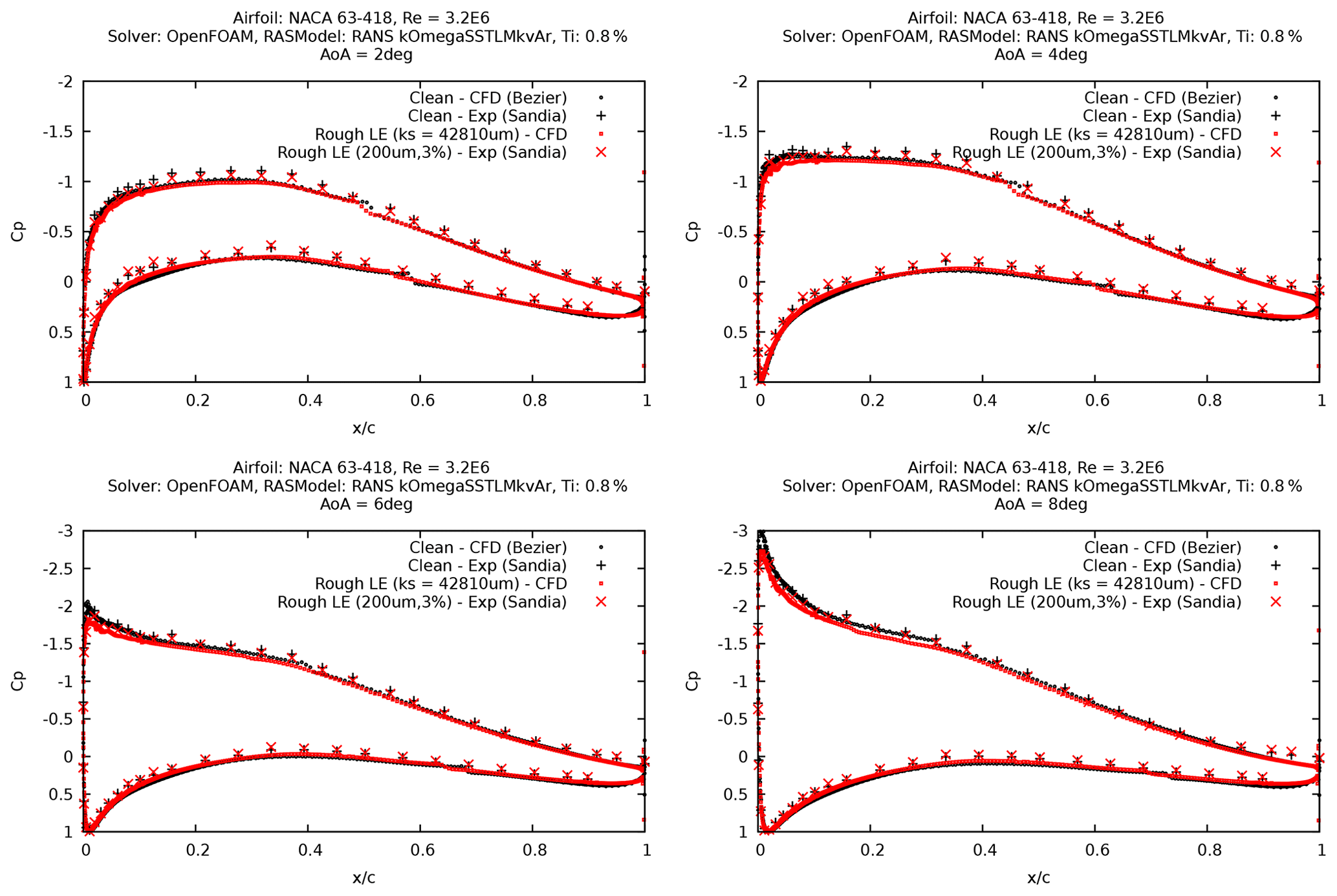
Figure 13 Pressure distribution at $Re=\mathrm{3.2}\times {\mathrm{10}}^{\mathrm{6}}$ for NACA 63-418 with LE roughness height of 200 µm and 3 % density.

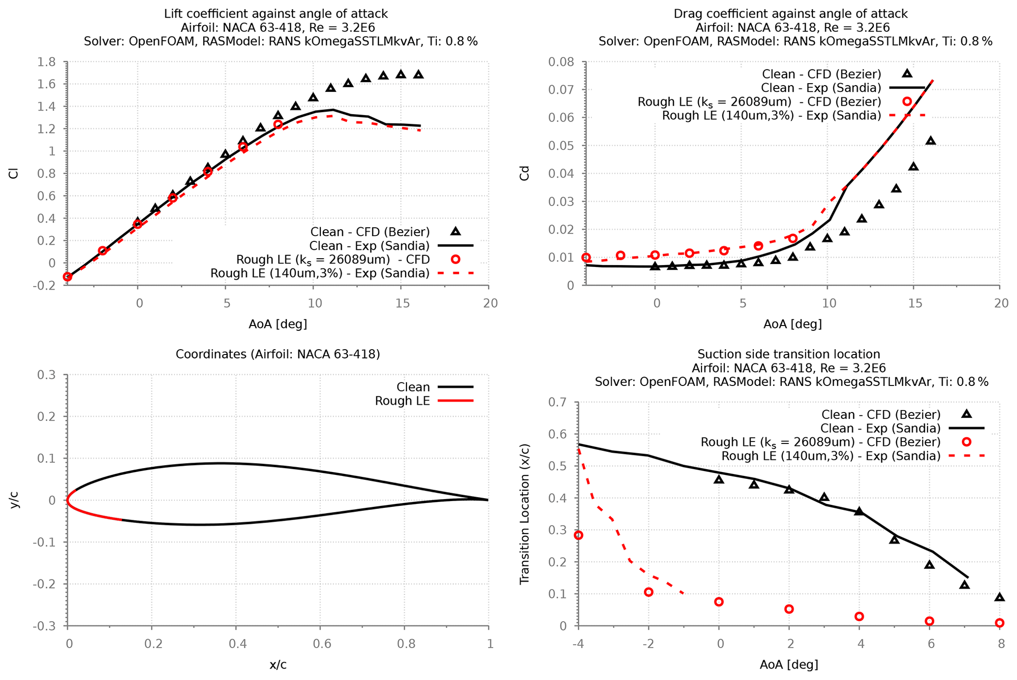
Figure 14 Calibration results at $Re=\mathrm{3.2}\times {\mathrm{10}}^{\mathrm{6}}$ for NACA 63-418 with LE roughness height of 140 µm and 3 % density.

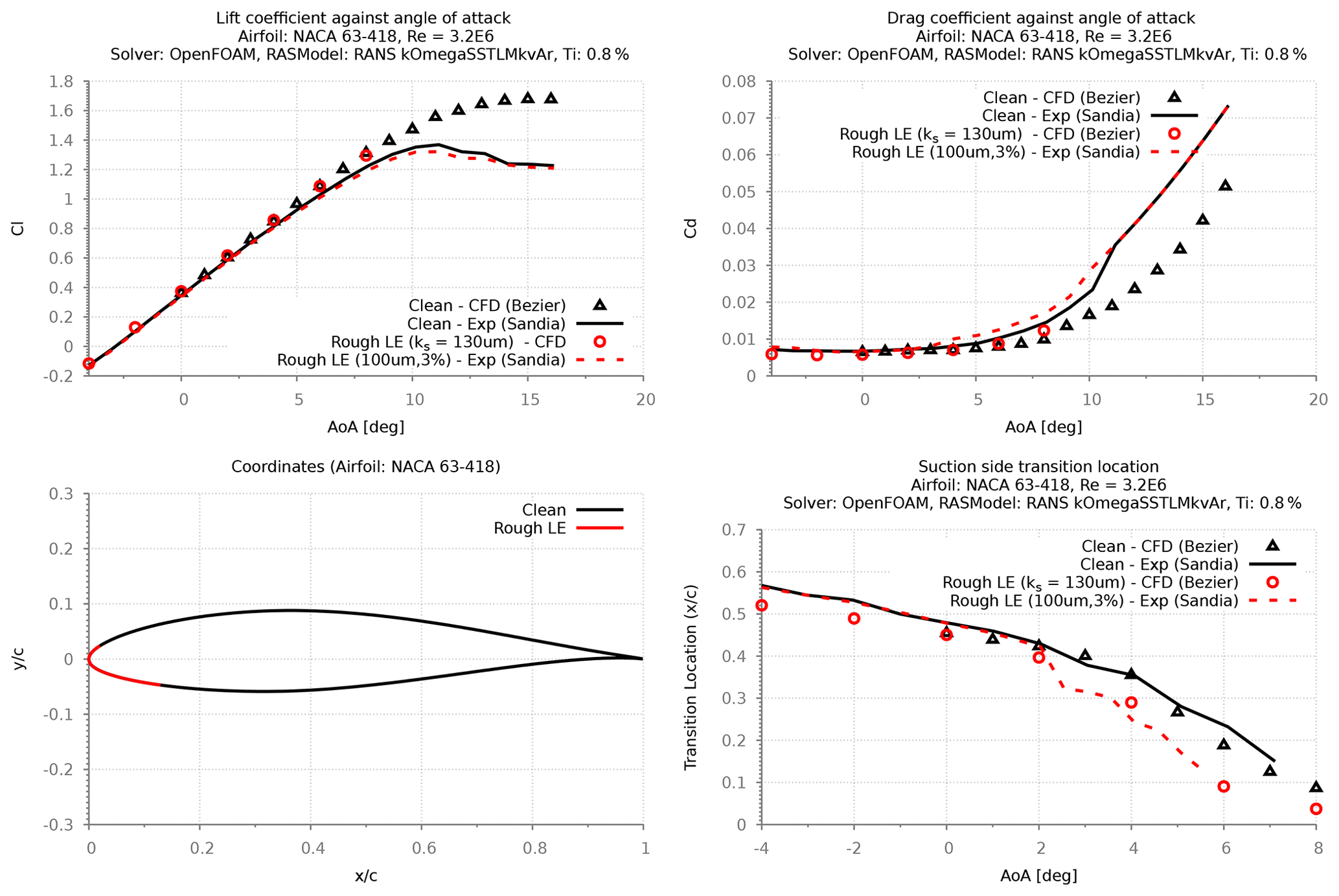
Figure 15 Calibration results at $Re=\mathrm{3.2}\times {\mathrm{10}}^{\mathrm{6}}$ for NACA 63-418 with LE roughness height of 100 µm and 3 % density.

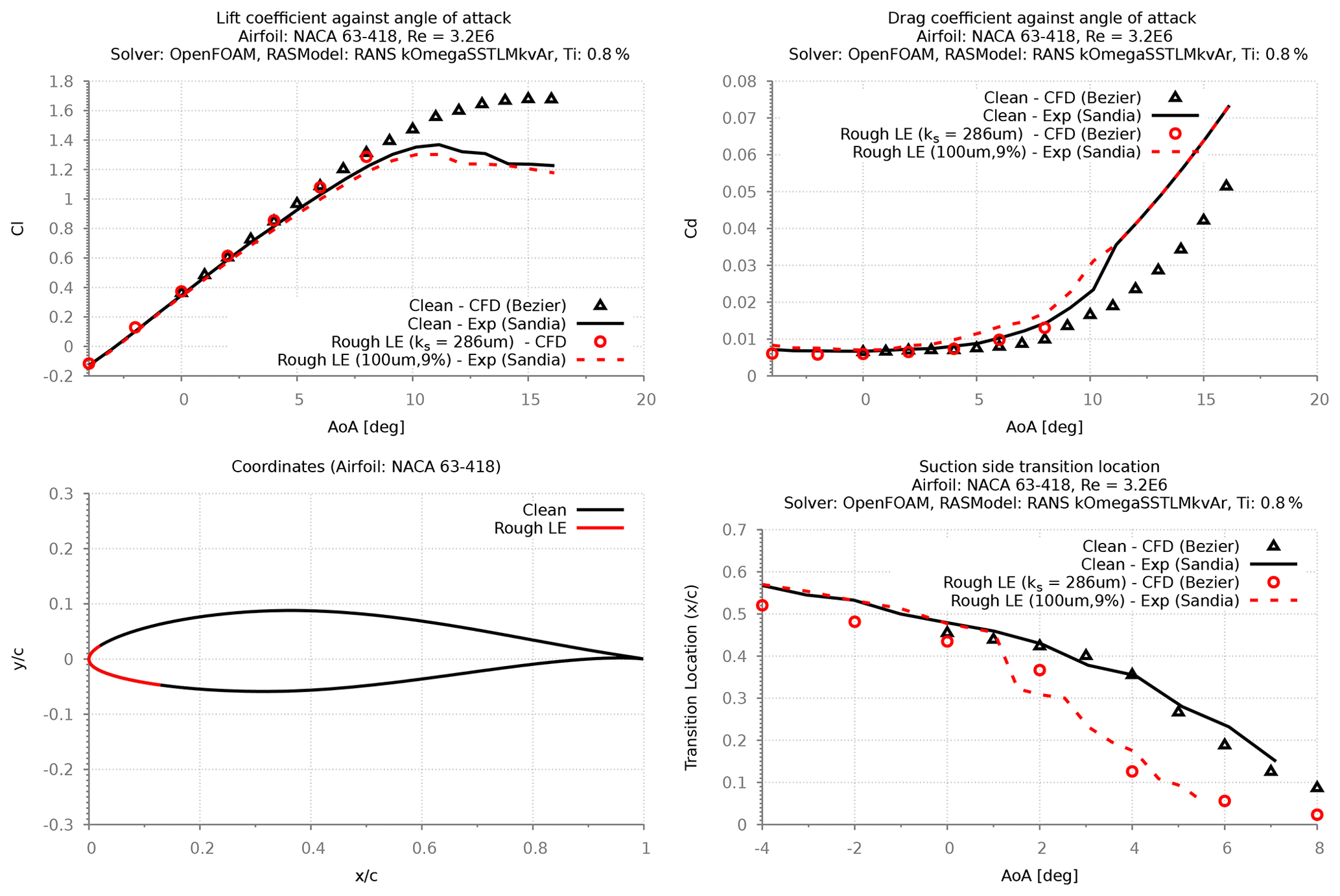
Figure 16 Calibration results at $Re=\mathrm{3.2}\times {\mathrm{10}}^{\mathrm{6}}$ for NACA 63-418 with LE roughness height of 100 µm and 9 % density.

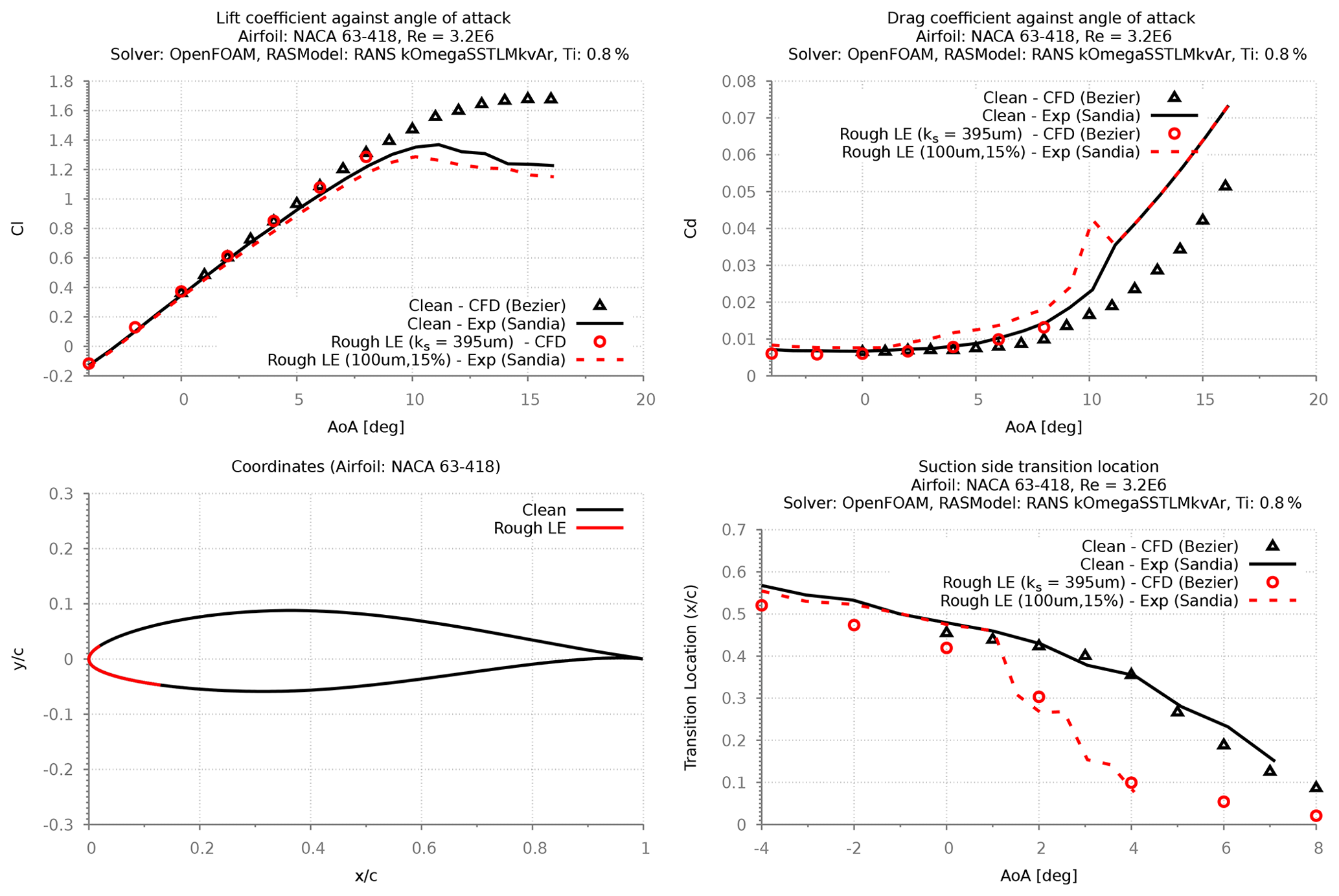
Figure 17 Calibration results at $Re=\mathrm{3.2}\times {\mathrm{10}}^{\mathrm{6}}$ for NACA 63-418 with LE roughness height of 100 µm and 15 % density.

The calibration study was conducted by using a cost function that minimizes the errors between the calculated and measured transition locations across the experimented range of angles of attacks (−4 to 6^∘). Transition location data were only available between −4 and 6^∘ within the LEES dataset; thus the rough airfoil simulations were limited within this range of angles of attack and not higher to reduce the extensive number of simulations for the calibration data. As a result, the following equation was established for k_s as a function of roughness height (R_h) and density (R_D). This calibration equation (Eq. 10) was explicitly used to generate the results presented in Figs. 12–17.

$$\begin{array}{}\text{(10)}& {\displaystyle }\mathrm{}\mathrm{}\mathrm{}\mathrm{}\mathrm{}\mathrm{}\mathrm{}\mathrm{}\mathrm{}\mathrm{}\mathrm{}\mathrm{}\mathrm{}\mathrm{}\begin{array}{rl}{k}_{\mathrm{s}}& =[\mathrm{1.49783}\times {\mathrm{10}}^{\mathrm{9}}\sqrt{\begin{array}{l}\mathrm{9.29170684919976}\times {\mathrm{10}}^{\mathrm{24}}{R}_{\mathrm{h}}\\ -\mathrm{9.24939916631901}\times {\mathrm{10}}^{\mathrm{26}}\end{array}}\\ & -\mathrm{2950.72}]\times [-\mathrm{0.768462}+\mathrm{5.46075}\times {\mathrm{10}}^{\mathrm{17}}\\ & \left.\times \sqrt{\begin{array}{l}\mathrm{3.16961301221313}\times {\mathrm{10}}^{\mathrm{32}}\times R_{\mathrm{D}}\\ +\mathrm{9.79025531790832}\times {\mathrm{10}}^{\mathrm{31}}\end{array}}\right]\end{array}\end{array}$$

Despite only calibrating the k_s values to match the measured transition locations, the results show a very good agreement between the modeled and the experimented drag forces, especially for the large roughness heights of 140 µm and 200 µm (Figs. 12 and 14). All modeled results showed notable differences (10 %) with the measured lift forces, where the relative reduction in lift due to the rough LE was captured well, while the absolute values were over-predicted. This is also evident when comparing the pressure distributions (Fig. 13), where the CFD model agrees well with the relative reduction in suction pressure that was observed in the measurements.

For the roughness height of 100 µm, the calibrated results showed reasonable agreement with the measured transition location. However, the corresponding results on the drag forces were under-predicted in comparison with the measured values. Due to the lack of experimental data, it was only possible to study the effect of roughness density at the height of 100 µm. The results from this study (Figs. 15–17) clearly show that the calibrated CFD model is able to calculate the forward movement of the transition point with increasing roughness density, while the corresponding effect on the drag forces is poorly predicted. These results indicate that the calibrated CFD model fails to predict the measured aerodynamic forces for small LE roughnesses (100 µm).

2.4 Discussion (Part 1)

An investigation to develop and implement a transport equation-based boundary layer transition model for rough surfaces was successfully completed. This implementation was carried out for the open-source CFD code OpenFOAM, which was then calibrated using an experimental study. Numerous verification and validation studies were performed to establish realistic results for predicting roughness-induced flow transition for wind turbine applications.

Based on this study, it is clear that the newly developed CFD model, calibrated with the measured transition locations, shows good agreement of the aerodynamic forces for airfoils with leading-edge roughness heights on the order of 140–200 µm. Despite matching the location of the transition point, the results indicate that for a smaller roughness height of 100 µm, the model fails to accurately predict the measured forces. It is also noted that the resultant CFD model based on the limited amount of measurement data is strongly tuned to the Sandia experiment, using the NACA 63–418 at the flow Re of 3.2 million, and its sensitivity to other airfoils at different flow Re is currently unknown. Thus, further tuning with validation using independent measurements is highly recommended, especially for modeling the effect of roughness density.

3 Aerodynamic performance of 3D scanned eroded wind turbine blades (Part 2)

The largest wind turbine blades (WTBs) are deployed offshore, where noise restrictions are lower and therefore tip speeds can be higher. This leads to increased damage on the WTB by LEE (Fig. 18), which is even a larger issue offshore than onshore in terms of expensive repair and maintenance (O&M) operations.

LEE has become a primary concern for the offshore wind industry. A detailed understanding of the mechanisms and prediction of LEE is one of the most important questions in developing wind turbine technologies and lowering the levelized cost of energy (LCoE). Also, LEE of WTBs is one of the most common reasons for the reduction of power generation by wind turbines.

Relatively small-sized damages on the surface of the WTB have an impact on the overall performance and therefore the energy yield of a wind turbine. The LEE damage of wind turbines leads also to an increase in drag coefficient and decrease in lift coefficient for higher angles of attack. The tip part of the blade, due to the higher speeds, contributes to the majority of the torque production; the last 15 % of the WTB radius for a multi-megawatt rotor can contribute up to 25 % of its total power production. However, the higher speeds also result in higher droplet impact velocity and the erosion rate at this part of the blade.

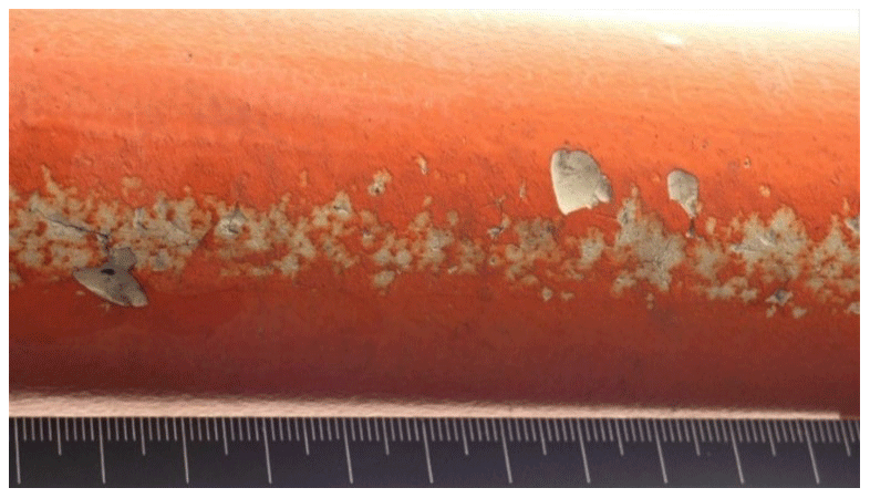
Figure 18 LEE damage on the tip section of a WTB, photographed by TNO.

Detailed understanding of the impact on aerodynamic performance due to the eroded LE is required to optimize the repair and operation, and accurate modeling tools are therefore essential. Damage mechanisms of LEE, 3D scanner technologies and CFD methods of modeling the erosion are discussed and presented; 3D images have added value for O&M purposes and quality control after repairing a WTB. Inspection and monitoring of a WTB are necessary to plan maintenance by keeping track of the degradation and structural health of the blade. In addition to visual inspection (manual or drone) the 3D scanning of the surface can be a suitable technique.

The novel aspect of this study is the modeling of high-resolution LE surface of the WTB with LEE damage, which was captured using state-of-the-art optical high-resolution 3D scanner technologies. This makes this research different from numerically assumed blades with LEE damage.

Using the point cloud data, 2D and 3D RANS CFD models have been applied to investigate the influence of shape change at the LE on aerodynamic performance. Both models are shown to predict the change in flow characteristics due to the LE differences. The results from CFD simulation have been used for BEM calculation to establish the performance of the WTBs in terms of power coefficient and relative changes in AEP. The AEP assessment was conducted using a mean wind speed of 10 m s⁻¹ with a Rayleigh wind distribution. A comparison of the simulation results is also made between two different CFD solvers.

3.1 LEE mechanism

LEE affects almost all wind turbines, and it has a harmful effect on the aerodynamic efficiency of the wind turbine blade, reducing the AEP, O&M cost, and the lifetime of the wind turbine. The energy losses associated with LEE on an operational wind farm are examined, with the average annual energy production dropping by 1.8 % due to medium levels of erosion, with the worst-affected turbine experiencing losses of 4.9 % (Law and Koutsos, 2020).

Another study shows results of an in-depth study indicated that a heavily eroded WTB can reduce annual energy production by up to 5 % for a utility scale wind turbine. Accounting for performance losses due to common blade surface roughness, such as dirt and insects, does not account for the increased performance loss due to the more severe surface roughness caused by the erosion of LE blade material (Ehrmann et al., 2017).

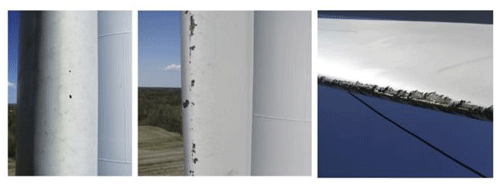
Figure 19 Changes to the LE surface due to impact with a different degree of severity. From left to right, LEE at an early stage, severely damaged coating and LEE starts to wear the shell material. Adapted from Keegan et al. (2013) and Rempel (2012).

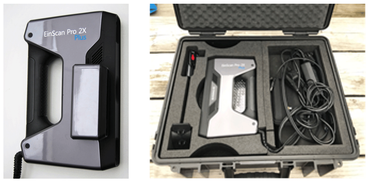
Figure 20 EinScan Pro 2X Plus Handheld 3D Scanner and the flight case with the equipment, photographed by TNO.

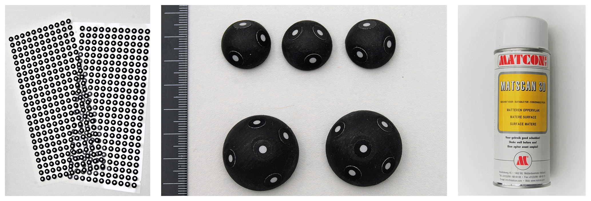
Figure 21 From left to right, 3D marker stickers, large spherical markers, 3D scan anti reflection spray, photographed by TNO.

Types of LEE and surface roughness (Slot et al., 2015) represented in Fig. 19 include the following:

1. An incubation period exists in which the surface is virtually unaffected. The roughness of the surface and small pit shaped defects in the coating will appear.

2. There is a steady-state erosive wear stage where the surface wears at a relatively high wear rate.

3. The final erosion stage possesses a strongly reduced wear rate due to the higher surface roughness which was produced in the second phase. Damage reaches the structural composite material of WTB.

That erosion has serious impacts on the rotor performance, which has been shown previously in a study at the University of Illinois where the DU 96-W-180 airfoil was tested in combination with a polyurethane wind protection tape. During the experiments, an increase in drag coefficient by 80 %–200 % was observed. Additionally, a decrease in lift coefficient for higher angles of attack was ascertained. The results also implied a significant loss in annual energy yield by 7 % for an increased drag coefficient of 80 %, which underlines the necessity of an independent, comparable and repeatable erosion test (Liersch and Michael, 2014).

The NREL5MW turbine (Jonkman et al., 2009) is simulated with clean and eroded blades, which are compared to coated blades equipped with LEP. Aerodynamic polars are generated by means of CFD, and load calculations are conducted using the BEM theory. The analysis in this work shows that, compared to clean rotor blades, the worse aerodynamic behavior of strongly eroded blades can lead to power losses of 9 %. In contrast, coated blades only have a small impact on the turbine power of less than 1 % (Schramm et al., 2017).

3.2 3D scanning technology for WTBs

Periodic replacement and maintenance of damaged WTBs leads to significant downtime and operational costs. The costs are mainly determined by the periodic repair of the leading edge coating or tape or even replacement of the complete WTB. The selection of the most suitable type of LEP (coating, tape, shell) depends also on the conditions the WTB is exposed to during the operational period (precipitation type and intensity, tip speed, UV, temperature). Currently, there are no maintenance-free WTB designs available and the high cost of the blades made it necessary to find new methods for inspection, monitoring and repair.

There are no references to any optical scanning systems that are already in practice for O&M of WTBs. Several innovative solutions have been developed for scanning WTBs in a controlled environment for production quality control. Amongst them, Aanæs et al. (2018) have described a complete autonomous inspection system for WTB surfaces. The measurement system presented here is composed of a high-resolution, structured light-based 3D scanner and a local positioning system. The locomotion system is composed of a six-axis industrial robot mounted on a mobile platform. It was found that a combination of a structured light 3D scanner and a laser tracker with an active target formed a good measurement system. The range of this system could be extended by an industrial robot mounted on a mobile platform. FORCE Technology and SGRE have developed an optical scan application with an autonomous robot for quality control of the WTB after production (Jensen, 2019).

Several different 3D hand-scanning tools are currently available on the market, and we can see a fast phase development for these technologies, as they are used for various applications ranging from small to larger scales, including scanning of the whole WTBs for quality assurance during production (Shining3D, 2018; Aanæs et al., 2018). For the study presented on this paper, the Shining3D EinScan Pro 2X Plus Handheld 3D Scanner was selected based on the performance, ease to use, and good price–quality relation (Fig. 20).

Figure 22 Prima pack add on plugged in the handheld scanner, photographed by TNO.

The handheld's rapid scan mode was used for the scanning of a WTB profile. For detailed scanning of a damage profile, like LEE damage, the high-definition handheld (HD scan) mode is recommended with maximum scanning accuracy of 0.05 mm. The HD scan mode requires the application of 3D markers on the surface (Fig. 21). The Prima pack add-on camera (Fig. 22) improves the capability to scan objects like a WTB surface without surface morphology and markings like 3D marker stickers, holes, ridges, lines, edges, etc. The experiments are performed by TNO in the field with different used WTBs and different conditions.

Table 2 Limitations and mitigating measures for scanning in outdoor conditions.

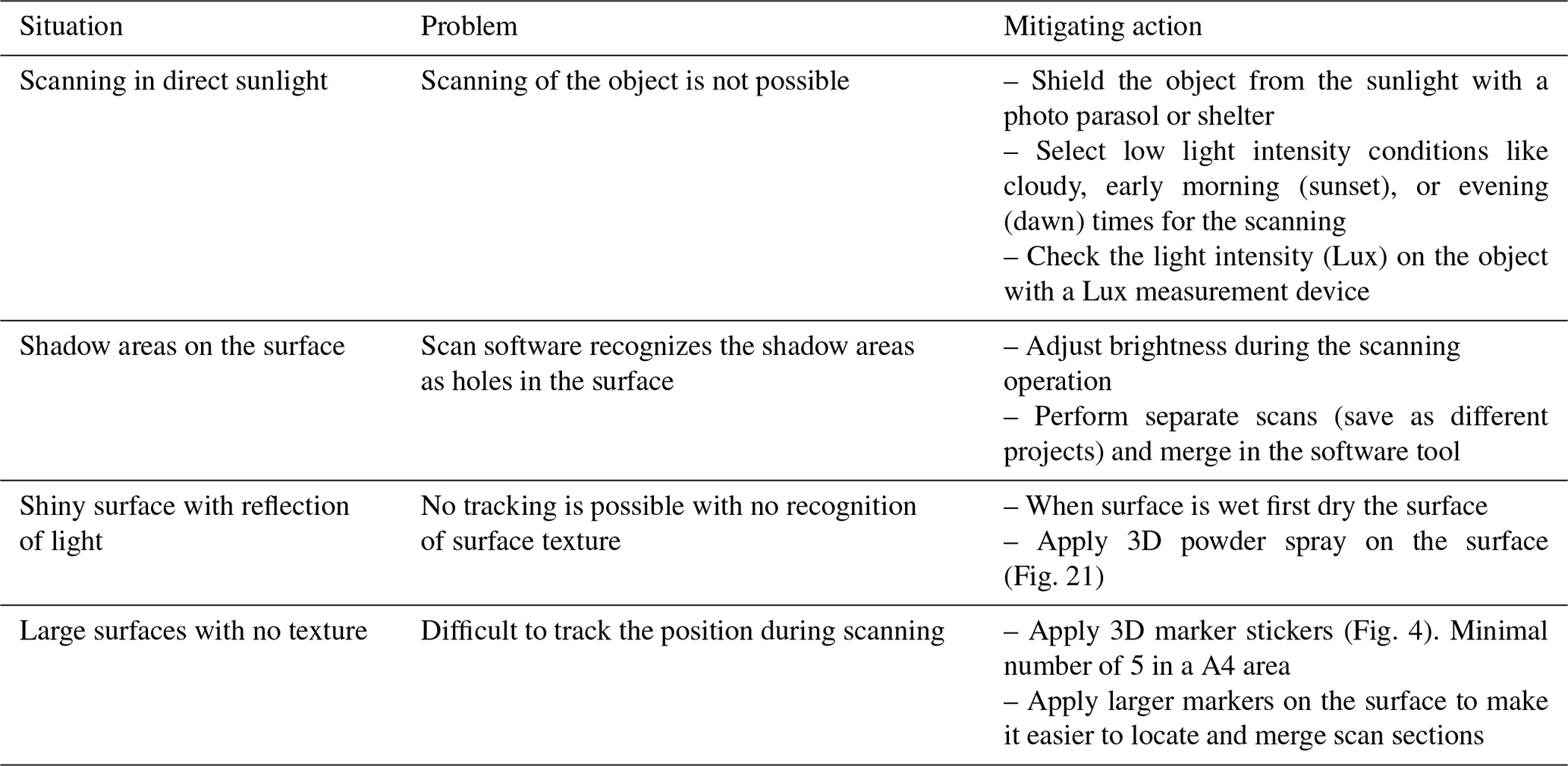
The EinScan Pro 2X Plus Handheld 3D Scanner as well as the flight case with the equipment is shown in Fig. 20. From left to right, one can see the 3D marker stickers, large spherical markers, and 3D scan anti-reflection spray, photographed by TNO. The EinScan Pro 2X Plus Handheld 3D Scanner is an optical scanner that restricts the usage environment. Too strong ambient light outdoors will affect the scanner light so that the light projected from the scanner will be hard to capture the data properly. Therefore, it is recommended to choose cloudy days or dusk when the light intensity has been reduced when scanning outdoors. For practical situations and problems, possible measures and solutions are given in Table 2.

Figure 23 3D scanning of a tip section of a WTB using sticker markers, photographed by TNO.

3.3 3D scanning of a WTB and conversion to CAD format

The applied 3D scan is performed at location Eemshaven, the Netherlands, on a research turbine with a blade radius of 63 m. The scan operation is performed in cloudy conditions with low ambient light intensity. For the high-resolution scan mode (0.05 mm resolution) the 3D marker stickers were applied on the surface (Fig. 23).

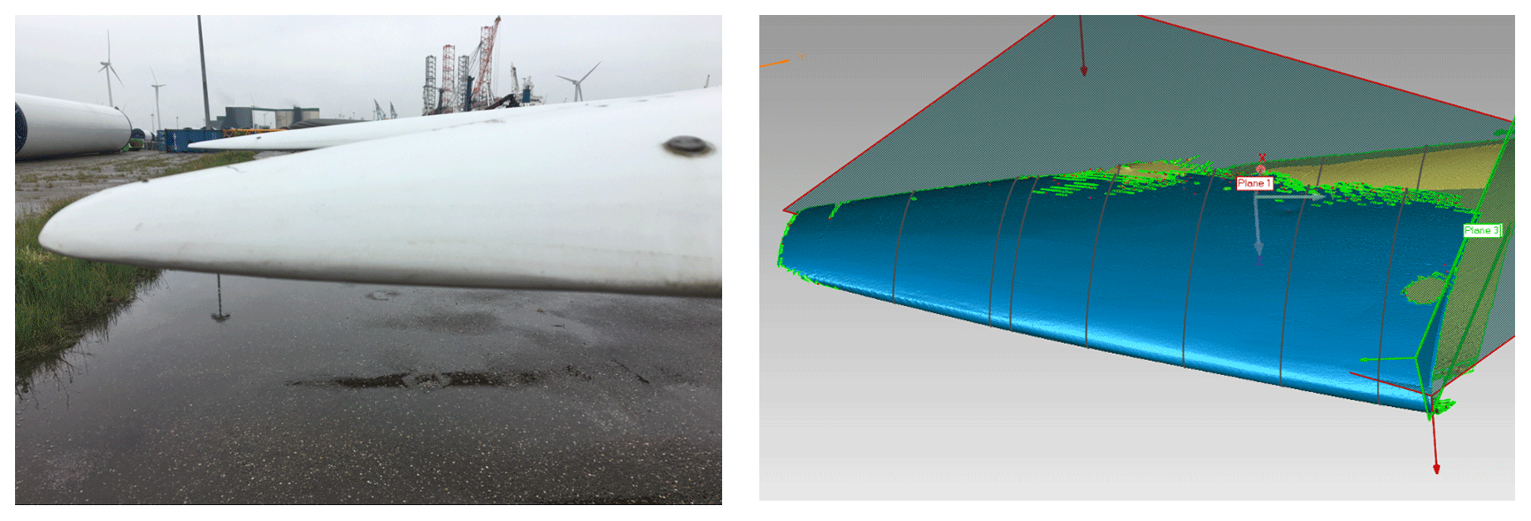
Figure 24 WTB tip (left, photographed by TNO) and the corresponding 3D point cloud image generated by TNO using the Geomagic Essentials tool.

For scanning objects with large curved surfaces, like a WTB, the fast handheld scan mode was utilized with the medium to low resolution with the Prima Pack add-on camera as described in Sect. 3.2 (Fig. 22). Tracking marker stickers were applied for regions where the scanner failed to recognize the surface characteristics (texture, color variation). For larger areas (>1 m²) multiple scans were necessary, which were then merged digitally into a single-point cloud image. Large 3D markers (Fig. 21) supported the scanning and merging of the large sections. An example of the WTB tip scanned with the fast scan mode without application of markers is shown in Fig. 24 and with the marker in Fig. 25.

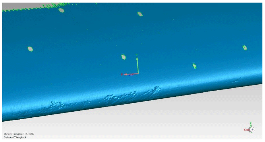
Figure 25 Screenshot generated by TNO of the meshed 3D point cloud imported in Geomagic Essentials 1 software tool. Green holes on the surface are the locations of the 3D sticker markers.

Figure 26 Screenshot generated by TNO of the processed watertight mesh model of the scanned LE.

The generated 3D point cloud is imported into the Geomagic Essentials 1 software tool (Fig. 25) and processed with the “Mesh doctor” tool to remove holes (3D markers), imperfections, and noise. The “watertight” mesh model (Fig. 26) must be transformed into a CAD format, *.IGS or *.STL, for application in CFD.

The *.STL file format is commonly used for digitalization, smoothing, and re-meshing of the 3D models. The imported database file (point cloud) of the scanned sections of the blade should be translated in *.SLDPRT file format. Then a new geometry file can be converted to *.IGS or *.STL format and imported to the “Pointwise” meshing tool.

Figure 27 DU97-W-300 airfoil coordinates.

3.4 CFD modeling of scanned LE

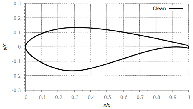
Several 2D and 3D numerical simulations were conducted to model the scanned surface of the eroded blade section. Two different steady RANS turbulence models were investigated for their relative differences in modeling eroded blades. One considers a fully turbulent boundary layer using Mentors SST turbulence model (Menter, 1994), while the other includes modeling of the laminar–turbulent flow transition using γ−Reθ_t correlation-based SST model (SSTLM) (Langtry, 2006). Both turbulence models were validated on the DU97-W-300 airfoil (Fig. 27) at the flow Re of 2×10⁶, based on the experimental data from Baldacchino et al. (2018).

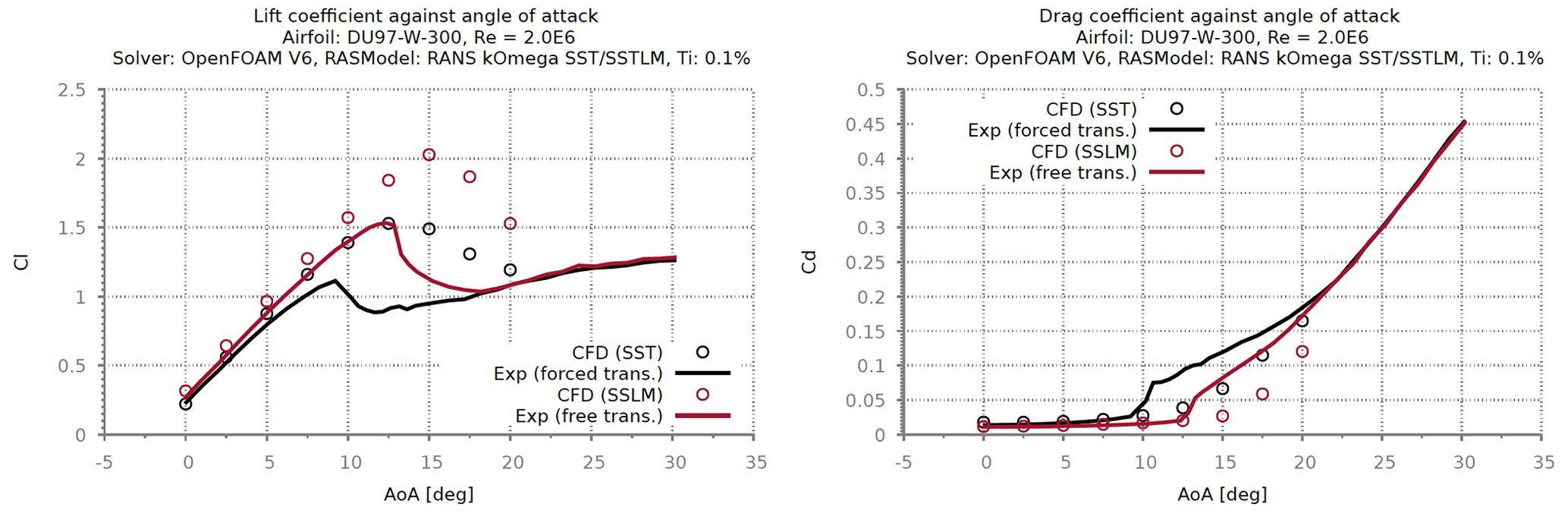
Figure 28 Validation of fully turbulent (SST) and transitional (SSTLM) lift and drag polar with experiment.

3.4.1 Validation study

The results from the validation study showed that both SST and SSTLM (Fig. 28) RANS CFD model captures the aerodynamic performances of a wind turbine section with reasonable accuracy at pre-stall (attached flow) conditions.

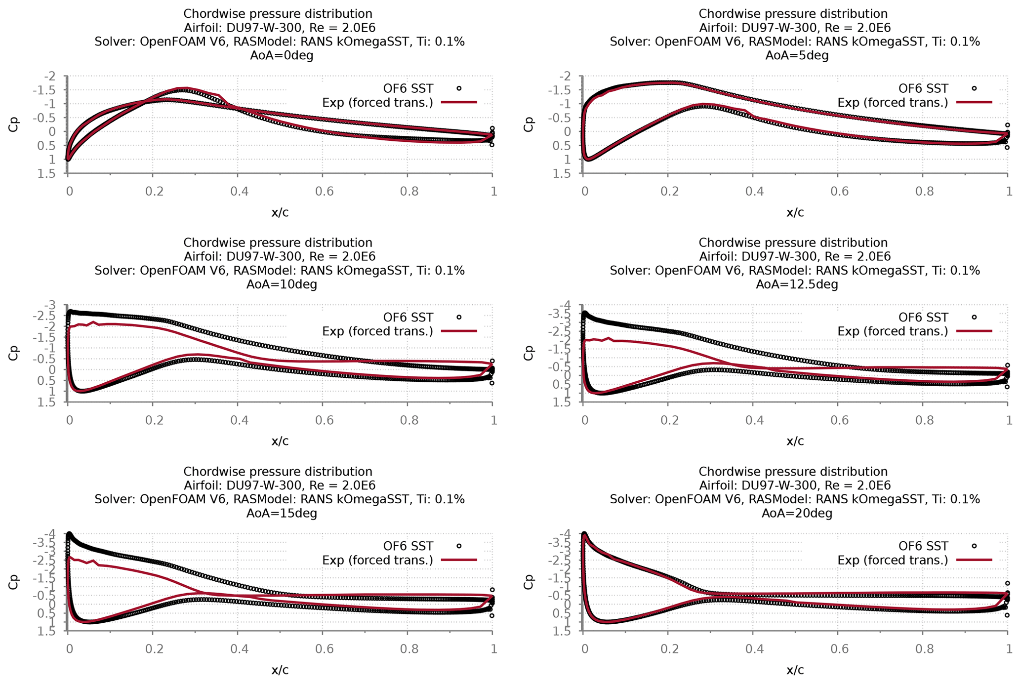
Figure 29 Chordwise pressure distribution comparison with experiment – forced transition/fully turbulent boundary layer (SST).

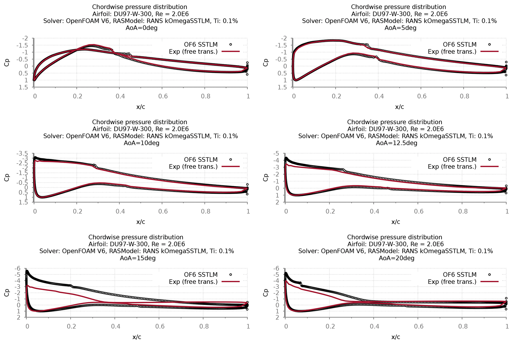
Figure 30 Chordwise pressure distribution comparison with experiment – free transition boundary layer (SSTLM).

A detailed validation study was conducted using surface pressure measurements for both turbulence models (Figs. 29 and 30). Based on the result it was also found that both CFD models concurrently calculate surface pressures that are in good agreement with the attached flow measurements.

The validation results indicate that the investigated CFD model is able to model the flow physics associated with fully turbulent boundary layer and flow transition and replicate the trends in lift and drag forces.

In comparison with experimental measurements, the computed clean airfoil lift and drag forces were validated within 10 % of the measurements (AoA: 0 to 7.5^∘). Unsteady computations may improve the validation at the large angles of attack. Nevertheless, based on the results it is clear that the relative changes in surface pressure and the trend in lift and drag forces for differing boundary layer conditions are captured with the chosen CFD model.

Figure 31 Selected portion of the scanned LE surface and its numerical grid.

3.4.2 Results from modeling 3D scanned surface

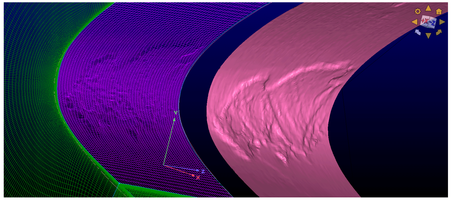
Using the validated CFD model a smaller portion of the scanned surface containing the worst part of the blade was discretized for the numerical simulation. A 3D study was performed to analyze the impact of erosion as scanned (Fig. 31). In parallel, a 2D sensitivity study was also conducted using the worst-eroded cross-section within this part to establish a correlation map between LEE against AEP.

The 2D mesh grid refinement studies were performed for the transitional analysis of the clean airfoil (Fig. 5). However, due to the limited computational resources, the 3D grid refinement study for the scanned eroded geometry was only performed with SST model. For the 3D simulations, two different grid densities were tested for grid-independent results. The first grid was constructed with 3 million hexahedral elements, with a resolution of 0.2 mm at the LE, while the fine grid was generated with 10 million hexahedral elements with a resolution of 0.1 mm at the LE. A span length of 6 % chord was used for this study, which was modeled with approx. 150 elements. In total, approx. 700 elements were used to model both suction and pressure sides of the airfoil, where 400 elements were dedicated purely to model the LE. The clean blade section was only modeled with 3 million elements for comparison. Slip/symmetry boundary conditions were used for the lateral walls of the domain.

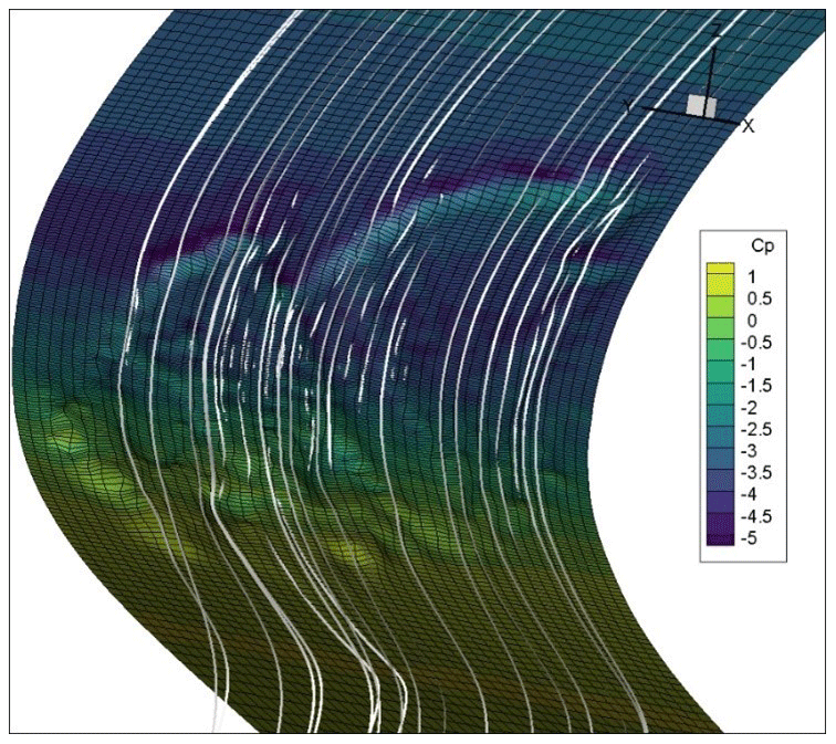
Figure 32 Pressure contours with flow ribbons at the eroded LE ($\mathrm{AoA}=\mathrm{10}{}^{\circ }$, SST, grid resolution: 3 million).

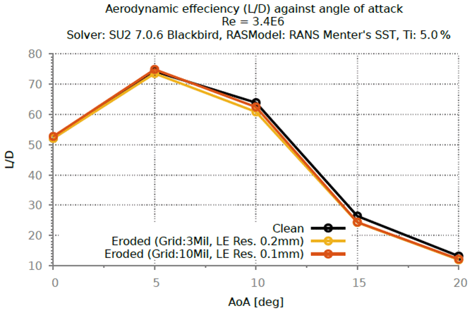
The results from the 3D simulations clearly show detailed pressure resolution across the degraded surface ($\mathrm{AoA}=\mathrm{10}{}^{\circ }$, Fig. 32). However, overall results show a negligible difference in the aerodynamic performance (Fig. 33) is expected under a fully turbulent boundary layer. It was also noticed that despite having inflicted local flow disturbances at the LE, the eroded surfaces showed a negligible effect on the flow downstream.

If the boundary layer is fully turbulent there is no shift in boundary layer transition point possible, which desensitizes a further change of LE shapes. This results in a minimal effect on the aerodynamic airfoil performance, thus resulting in negligible difference to AEP. However, this is true within the limited degree of LE shape change studied within this investigation. A very substantial change of airfoil shape will have an impact on the pressure distribution and so will likely influence the airfoil performance.

Figure 33 Lift-to-drag ratio comparison between clean and eroded blade section.

3.4.3 Results from 2D sensitivity study

A sensitivity study was carried out using a 2D profile extracted from the scanned 3D LE (Fig. 34), and then two more artificial profiles were generated by simply performing a lateral translation of the extracted LE towards the trailing edge. The translation distance was calculated based on the maximum lateral difference between the clean and eroded LE (Fig. 35), which was found at $x/c$ and $y/c$ corresponding to (0,0). This distance of 0.26 %c was then multiplied by 2 and 3 to generate the eroded 2x and 3x profiles. These relative LE differences were then superimposed on a generic WTB tip airfoil NACA64-618, specifically the NREL5MW reference turbine for the assessment of AEP.

Figure 34 Extracted profile for 2D sensitivity study.

Figure 35 Superimposed eroded LE change for NACA64-618.

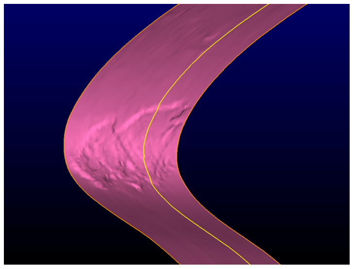
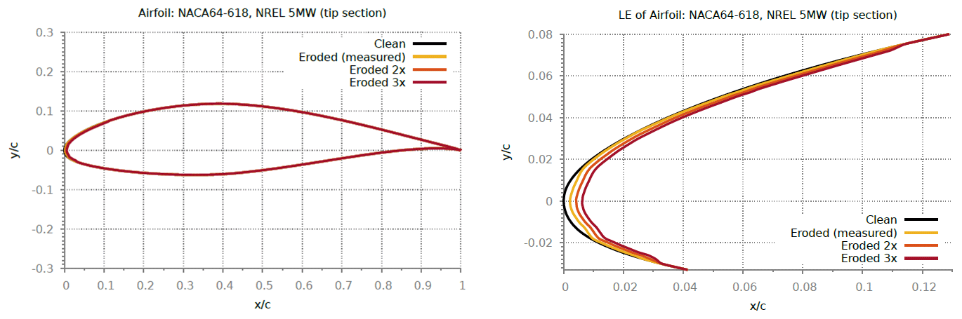
Table 3 NREL5MW blade definition (r – local radius in m, R=63 m, c – chord).

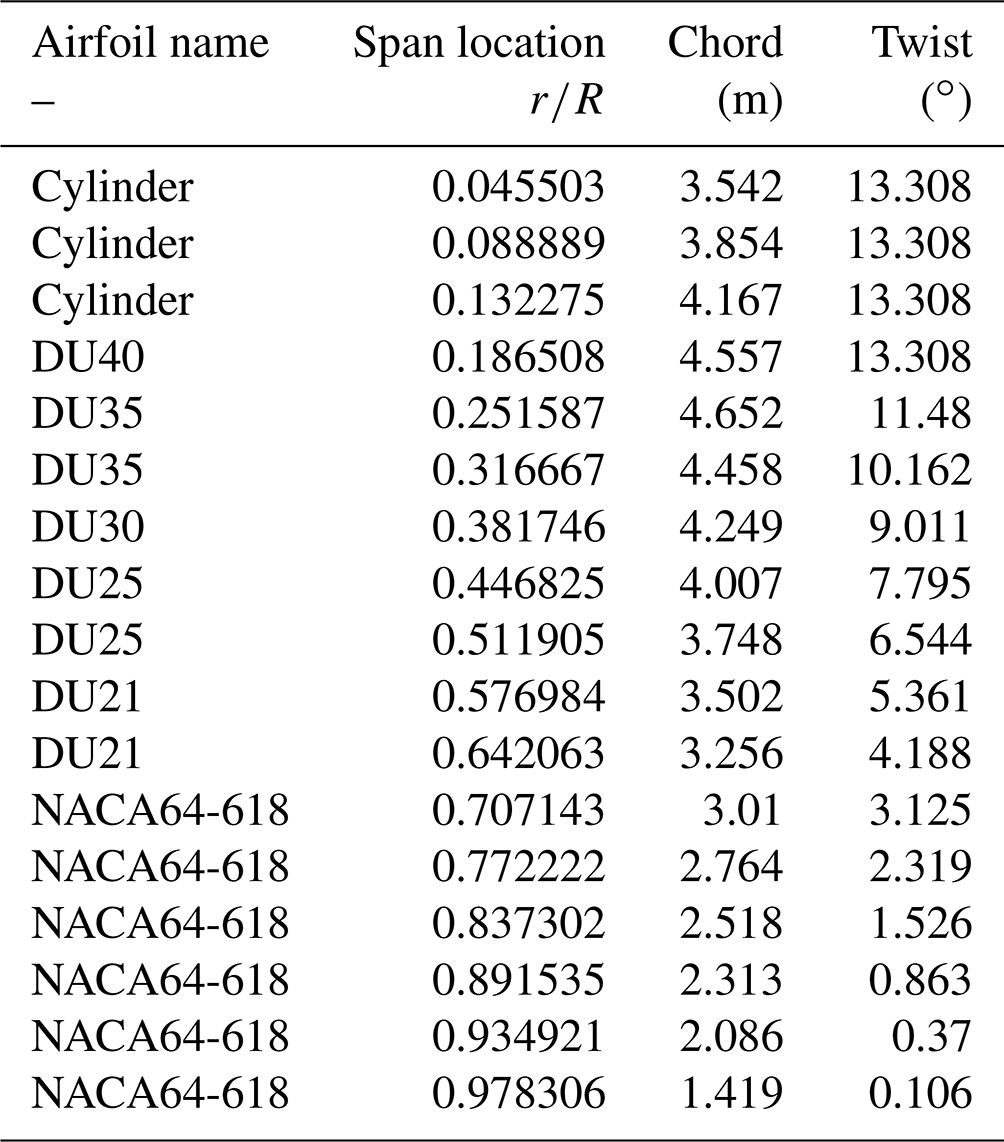
Figure 36 2D lift and drag coefficient sensitivity against angle of attack for NACA64-618 section (a, b SST, c, d SSTLM).

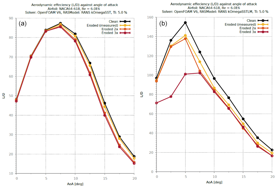
Figure 37 2D lift-to-drag ratio sensitivity against angle of attack for NACA64-618 section (a SST, b SSTLM).

Table 4 Relative change (compared to SSTLM clean) in AEP of NREL5MW rotor with Rayleigh 10 m s⁻¹ mean wind speed, under transitional condition considering different degrees of LEE for different tip span extents.

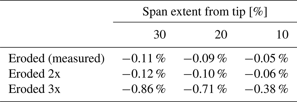
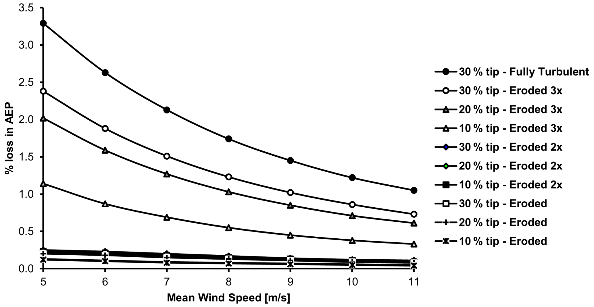
Figure 38 Percentage loss in AEP of NREL5MW turbine considering different degrees of LEE for different tip extents.

The details of the BEM framework used for this work are documented in Vimalakanthan (2014). Using the same BEM model for NREL5MW blade (Table 3) the tip airfoil NACA64-618's polar data were changed at different radius intervals to study the effect of erosion for different tip extents. For instance, the case of 30 % eroded tip with the largest LEE was calculated by replacing all NACA64-618 sectional polar data from Table 3 with the eroded 3x data from Fig. 36.

The results from this investigation also suggest that under fully turbulent conditions the investigated LE shapes show the least amount of influence on the aerodynamic performances (Fig. 36) and results in a negligible difference to AEP of the NREL5MW rotor (−0.02 %, eroded 3x up to the last 30 % of blade radius).

Under a transitional flow environment, results show a much larger aerodynamic impact due to the investigated shape changes at the LE. The results show up to 50 % reduction in aerodynamic efficiency (Fig. 37) even at the lower angles of attack, when the shape of the LE degrades by 0.8 % of the chord (eroded 3x). Based on transition modeled results, the BEM investigation examining different span extents (Table 4) of erosion has revealed up to 0.86 % reduction in AEP when the LE shape is changed by 0.8 % of the chord for the last 30 % of the blade span. However, if a lower mean wind speed is considered for the wind distribution, the AEP loss is calculated to be much higher (Fig. 38). This clearly indicates that the relative AEP loss from erosion is much higher for turbines with a low-capacity factor and vice versa for a high-capacity factor as the turbines operate at mostly above-rated conditions, where there is no loss from erosion.

3.5 Discussion (Part 2)

Based on the research conducted with the EinScan Pro 2X Plus Handheld 3D Scanner, the method has been shown to be suitable for generating the 3D point cloud data input of WTB surfaces for CFD analysis. There are limitations to outdoor scanning conditions where direct sunlight and shadows on the surface will disturb or make scanning of the surface with this LED scanner impossible. Mitigating measures include shielding from direct sunlight (shelter or parasol) and scanning at low light intensity, such as sunrise, sunset or cloudy conditions. The 3D scan method can be applicable for O&M on WTBs. In addition, to inspect and monitor LEE damage, other types of failure mechanisms can also be included that result in changes in the WTB profile. Examples of WTB damage are sand erosion, surface cracking and lightning strike damage.

The CFD models have clearly shown to predict the change in flow characteristics due to the LE differences. The results from CFD simulation have been used for BEM calculation to establish the performance of the WTBs in terms of power coefficient and relative changes in AEP. Comparisons of the simulation results were also made between two different turbulence models. Based on the results it was found that under fully turbulent flow conditions the investigated shape difference at LE has negligible differences in aerodynamic performance. However, when flow transition is modeled, the results show a significant impact on aerodynamic efficiency. BEM investigation examining different span extents of erosion for the NREL5MW rotor has revealed that up to 0.86 % reduction in AEP can be expected when the LE shape is changed by 0.8 % of the chord. It is noted that the aerodynamic modeling adapted for this work does not account for differences due to surface texture and has only modeled the shape change due to LEE, and if considering the effect of flow transition being trigged by the surface textural difference due to LEE, then a larger reduction in AEP was calculated (−1.24 %). It is also noted that if the turbine operates mostly in the sub-rated region of the power curve or is placed at a low wind site (low-capacity operation), a much larger AEP loss (−3.3 %) is realized due to LEE.

Although the generated grid resolution was made to capture numerical details on the order of 0.1 mm, the RANS turbulence modeling approach used in this study inherently poses uncertainty for capturing flow details at this scale of changes in geometry. The steady RANS modeling was chosen due to its computational efficiency and to meet the project time constraints. Despite RANS being considered an industry standard and quite accurate for many flow problems, the results may differ when a higher-order turbulence model such as large eddy simulation (LES) or a hybrid RANS–LES models is used to model these fine geometrical details.

Overall, this investigation to evaluate the aerodynamic impacts due to actual LEE has been successfully completed. Based on the results, it was established that under the assumptions of this work, considering pure shape changes in LE of the tip part of the blade for a 5 MW wind turbine can reduce its AEP on the order of 3.3 %. However, if the effect of the exposed fibrous blade material on the transitional boundary layer was included using a model like the one described in Part 1, it will further deplete the sectional $L/D$ ratios, thus resulting in further loss in AEP.

4 Conclusions

LEE is one of the most critical degradation mechanisms that occur with WTBs, generally starting from the tip section of the blade. A detailed understanding of the LEE process and the impact on aerodynamic performance due to the damaged LE is required to select the most appropriate LEP system and optimize blade maintenance. Providing accurate modeling tools is therefore essential.

Based on this two-part study, the investigation of different orders of magnitudes in erosion damage has shown that up to a 0.86 %–1.24 % reduction in AEP can be expected when the LE shape is degraded by 0.8 % of the chord, based on the NREL5MW turbine considering 10 m s⁻¹ mean wind speed Raleigh wind distribution. However, for low-capacity operations such as operating mostly in the sub-rated region of the power curve or being placed at a lower mean wind speed site, a larger reduction in AEP is calculated due to LEE (2.4 %–3.3 %). The results also suggest that under the fully turbulent condition the investigated LE shapes show the least amount of influence on the aerodynamic performances and result in a negligible difference to AEP. The present CFD model for modeling flow transition accounting for roughness shows good agreement of the aerodynamic forces for airfoils with leading-edge roughness heights on the order of 140–200 µm while showing poor agreement for smaller roughness heights on the order of 100 µm. It is also noted that the resultant CFD model based on the limited amount of measurement data is strongly tuned to the Sandia experiment, using the NACA 63-418 at the flow Re of 3.2 million, and its sensitivity to other airfoils at different flow Re is currently unknown. Thus, further tuning with validation using independent measurements is highly recommended, especially for modeling the effect of roughness density.

Appendix A: Abbreviations

AEP	Annual energy production
BEM	Blade element momentum
Cd	Coefficient of drag
CFD	Computational fluid dynamics
Cl	Coefficient of lift
LCoE	Levelized cost of energy
LE	Leading edge
LEE	Leading edge erosion
LEP	Leading edge protection
LES	Large eddy simulation
O&M	Operations and maintenance
RANS	Reynolds-averaged Navier–Stokes
Re	Reynolds number
SST	k−ω shear stress transport fully turbulent turbulence model
SSTLM	k−ω shear stress transport with Langtry–Menter transition turbulence model
SSTLMkvAr	k−ω shear stress transport with Langtry–Menter transition turbulence model including amplification factor formulation for wall roughness
Ti	Turbulence intensity
WTB	Wind turbine blades