the Creative Commons Attribution 4.0 License.
the Creative Commons Attribution 4.0 License.
 | 19 Mar 2021
Validation of the dynamic wake meandering model with respect to loads and power production
Inga Reinwardt
Levin Schilling
Dirk Steudel
Nikolay Dimitrov
Peter Dalhoff
Michael Breuer
The outlined analysis validates the dynamic wake meandering (DWM) model based on loads and power production measured at an onshore wind farm with small turbine distances. Special focus is given to the performance of a version of the DWM model that was previously recalibrated at the site. The recalibration is based on measurements from a turbine nacelle-mounted lidar system. The different versions of the DWM model are compared to the commonly used Frandsen wake-added turbulence model. The results of the recalibrated wake model agree very well with the measurements, whereas the Frandsen model overestimates the loads drastically for short turbine distances. Furthermore, lidar measurements of the wind speed deficit as well as the wake meandering are incorporated in the DWM model definition in order to decrease the uncertainties.
- Article
(7098 KB) - Full-text XML
- BibTeX
- EndNote


Wake models are a key aspect in every site-specific load calculation procedure. The used wake model has significant impact on predicted loads and the power output of the whole wind farm; hence, an accurate wake model is of major importance for a wind farm design optimization process. Planning a new wind farm is a highly iterative process, where time-consuming calculations are avoided as much as possible, so the complexity and the accuracy of the model need to be well balanced.
Simple analytical wake models can be divided into models estimating either the mean wind speed reduction in the wake or the wake-induced turbulence. While the former serves as a basis for power calculations, the latter is necessary to compute loads. One of the main simple analytical models for calculating the wake-induced turbulence in a wind farm is the so-called Frandsen model (see, e.g., Frandsen, 2007). Reinwardt et al. (2018) and Gerke et al. (2018) have shown that this model delivers conservative results, especially for short turbine distances, a limitation that is critical for onshore wind farms in densely populated areas, where a high energy output per utilized area is crucial. Another simple, but less common, analytical model to calculate the wake-induced turbulence is introduced in Quarton and Ainslie (1989). Jensen (1983) provides an analytical model to predict the wind speed reduction in the wake. More recently developed wind speed reduction models can be found in Larsen (2009) and Bastankhah and Porté-Agel (2014). The latter is based on a Gaussian distribution for the velocity deficit in the wake. A more sophisticated model for calculating the wind speed deficit expansion in the wake is explained in Ainslie (1988), where the author suggests to solve the thin shear layer approximation of the Navier–Stokes equations with an eddy viscosity closure approach.
The dynamic wake meandering (DWM) model investigated here is strongly influenced by the work of Ainslie (1988). It describes the physical behavior of the wake more precisely, while it is still less time consuming and complex than a complete computational fluid dynamic (CFD) simulation. Moreover, it is capable of estimating the wake-induced turbulence as well as the wind speed deficit. The model assumes that the wake behaves like a passive tracer; i.e., the wake itself moves in vertical and horizontal directions (Larsen et al., 2008b). The meandering motion in combination with the shape of the wind speed deficit in the meandering frame of reference (MFR) lead to increased turbulence at the wake-affected turbine and thus play an eminent role for the loads of the downstream turbine. As of late, the DWM model is included in the new edition of the International Electrotechnical Commission (IEC) guideline (IEC 61400-1 Ed.4, 2019). It was validated and calibrated with actuator disk and actuator line simulations as outlined in Madsen et al. (2010), whereas a validation of the model with measured loads and power production was carried out in Larsen et al. (2013). Keck (2015) presents a power deficit validation of a slightly different version and extension of the model towards a stand-alone implementation.
The DWM model has proven to be more accurate in load prediction than the commonly used Frandsen wake-added turbulence model (Reinwardt et al., 2018). Furthermore, Reinwardt et al. (2020) present a recalibrated version of the model, which provides a very precise description of the wind speed deficit in the MFR. The authors investigate the impact of the ambient turbulence intensity (TI) on the eddy viscosity definition in the description of the wind speed deficit in the MFR based on lidar measurements from a wind farm to determine an improved correlation function. The same wind farm is used in the present study. In the following analysis, the recently calibrated version of the DWM model is validated with respect to loads and power production and compared to the original model definition. A further analysis of the recalibrated model beyond the wake wind deficit is necessary to investigate the influence of the recalibration on loads and power production.
Besides the validation of the recalibrated model according to power output and loads, in the present study, lidar wake measurements are integrated into the load simulation to support the calculation and decrease the uncertainties. The measured wind speed deficit in the MFR and the time series of the meandering are introduced successively. Related studies with a different approach of integrating the lidar measurements are Dimitrov et al. (2019) for wake-free inflow conditions and Conti et al. (2020) for wake conditions. In comparison to the outlined methods, the approach investigated here does not need any high-frequency or raw data from the lidar system. It is purely based on the measured line-of-sight (LOS) wind speed. Furthermore, the outlined analysis focuses on the measured wind speed deficit and the meandering of the wake, which is successively introduced in the DWM model definition, whereas in Conti et al. (2020) special focus is given to the estimation of turbulence in the wake. The wake turbulence is only indirectly captured here by the investigated wake meandering and the wind speed deficit gradient in the MFR. The wake meandering together with the wind speed deficit gradient have a very high impact on the loads of the downstream turbine, so a more accurate description in the DWM model with the help of the lidar measurements has high potential to decrease the uncertainties in load simulations and thus is worth being investigated.
Hereafter, in Sect. 2, a detailed description of the examined wind farm as well as the installed measurement equipment is presented. The filtering and processing of the measured data are explained in Sect. 3. Section 4 introduces the load simulation software. A specification of the used models as well as the procedure of incorporating the lidar measurements into the model are given in Sects. 5 and 6. The document will be completed with the discussion of the results in Sect. 7 and a brief summary in Sect. 8.
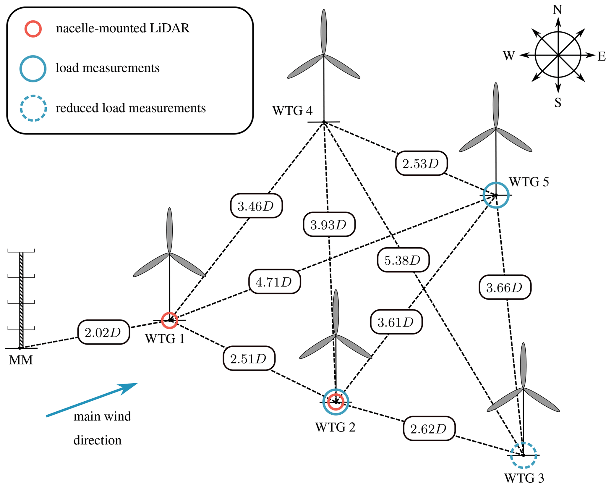
Figure 1Wind farm layout with measurement equipment (Reinwardt et al., 2020).
The analyzed wind farm is located southeast of Hamburg, Germany. The terrain is mostly flat, and no further wind farms are located in the immediate vicinity. Only at a distance of more than 1 km the terrain becomes slightly hilly (approximately 40 m difference in altitude). The distance to the next wind farm is approximately 3 km. The wind farm layout is depicted in Fig. 1. It includes five closely spaced Nordex turbines (1× N117 3 MW and 4× N117 2.4 MW). All turbines have a hub height of 120 m. An IEC-compliant 120 m met mast (IEC 61400-12-1, 2017) is placed in main wind direction ahead of the wind farm. It is equipped with 11 anemometers, two of which are ultrasonic devices, three wind vanes, two temperature sensors, two thermohygrometers and two barometers. The sensors are distributed along the whole met mast as depicted in Fig. 2. Furthermore, the turbine nacelles of wind turbine generator (WTG) 1 and WTG 2 are each equipped with a pulsed scanning lidar system (Galion G4000) with a pulse repetition rate of 15 kHz and a ray update rate of 1 Hz (depending on the atmospheric conditions), so that an average value of approximately 15 000 pulses is used per sample. The laser frequency is at 100 MHz. Considering the speed of light, this delivers a pulse length of 1.5 m. Hence, with a range gate length of 30 m, 20 points are used per range gate. Both lidar systems face downwind as depicted in Fig. 2. The device on WTG 2 is installed on top of the nacelle, whereas the device on WTG 1 is installed inside the nacelle, measuring through a hole in the rear wall. The unusual location derives from the fact that a heat exchanger on top of the nacelle occupies the essential mounting area. Additionally, nacelle-mounted differential GPS systems help tracking the nacelle's precise position with a centimeter range accuracy so that yaw movements can be calculated.
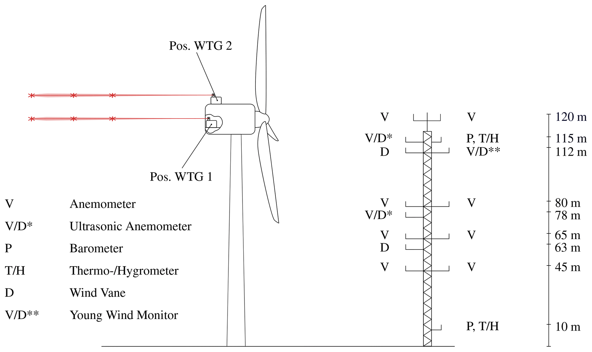
Figure 2Met mast (MM) measurement equipment and lidar positions (Reinwardt et al., 2020).
Lastly, at three turbines, load measurement equipment is installed. The tower top and bottom as well as blade flapwise and edgewise bending moments are measured with strain gauges at WTG 2 and WTG 5. WTG 3 is only equipped with strain gauges at the tower. The strain gauges at the tower top are installed 3.4 m below the nacelle and the strain gauges at the tower bottom are placed 1.5 m above the floor panel. The edgewise and flapwise moments are measured at a distance of 1.5 m from the blade root. Besides the installed measurement equipment, the turbine's supervisory control and data acquisition (SCADA) system is used to determine the operational conditions of the turbines.
Table 1Considered wind direction sectors for wake-free inflow and analyzed wake sectors.
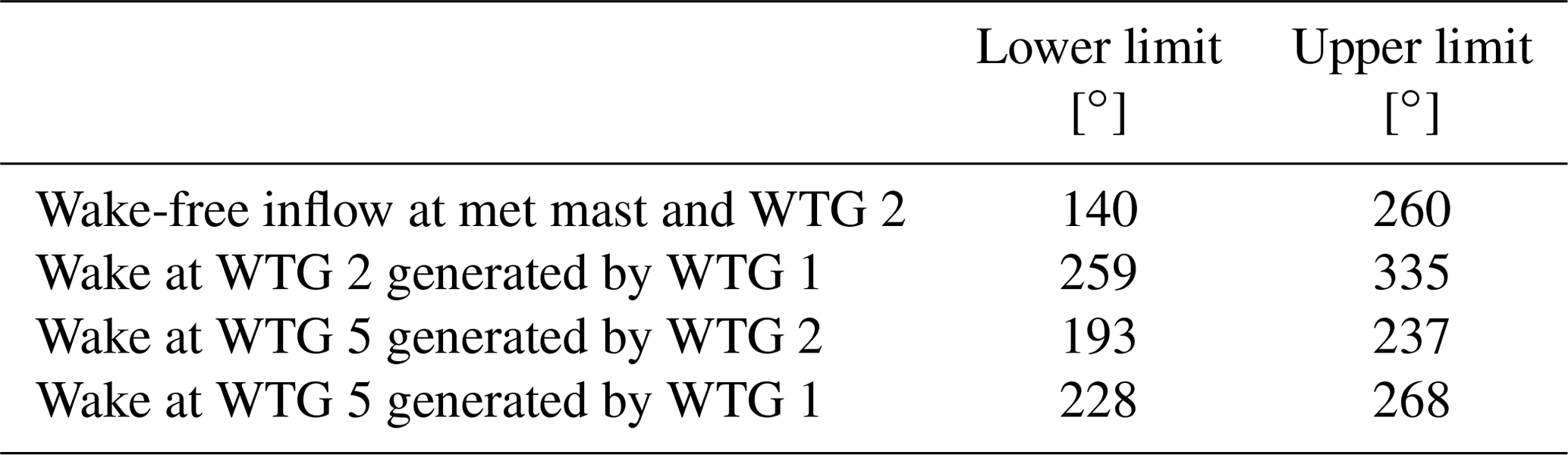
Measurement results from April 2019 to May 2020 have been used in the analysis. The data are filtered and sorted in accordance with the ambient conditions (e.g., ambient wind speed, turbulence intensity and wind direction) determined by the met mast and the operational states of the turbine tracked by the SCADA system so that all filtering is based on 10 min statistics from the met mast or the SCADA system. Only measurement results where the turbines operate under normal power production are included in the analysis. In the night, the turbines work in a reduced mode for noise-reduction purposes, so no data could be gathered during the night. The wind direction sectors for free inflow and wake conditions are summarized in Table 1. The filtering procedure leads to a large decrease of available data sets, so that, for example, at a turbulence intensity of 6 % and an ambient wind speed of 6 m s−1, only about 100 10 min data sets could be collected when WTG 2 is placed in the wake of WTG 1. Considerably more data sets could be collected for wake-free inflow conditions. In total, around 370 samples could be collected at a turbulence intensity of 12 % in the analysis in Sect. 7.1.
The measured lidar data are filtered by the power intensity from the returned laser beam, which is closely related to the signal-to-noise ratio (SNR) of the measurements. Furthermore, the scan time is observed, so only results with a sufficient scan time to track the wake meandering are considered. Lidar systems measure the LOS velocity. The wind speed in the downstream direction is calculated from the lidar's LOS velocity and the geometric dependency of the position of the laser beam relative to the main flow direction as outlined in Machefaux et al. (2012). Thus, the horizontal wind speed is defined as
where θ is the azimuth angle and ϕ the elevation angle of the lidar scan head. This approach is suitable for small scan opening angles of the scan head like in the measurement campaign presented here. The lidar system is capable of scanning a two-dimensional wind field in different downstream distances simultaneously. Here, the purpose of the lidar system is to capture the meandering and to estimate the wind speed deficit in the MFR. To ensure that the meandering as well as the wind speed deficit in the horizontal meandering frame of reference (HMFR) can be covered, a horizontal line is scanned instead of a full two-dimensional wind field. The one-dimensional scan consists of only 11 scan points scanned in a horizontal line from to 20∘ in 4∘ steps. Measurements were collected up to a downstream distance of 750 m in 30 m steps. The duration of the horizontal line scan is usually about 16 s depending on the visibility conditions during the scan. At poorer conditions, the scan can take up to 25 s.
The loads are simulated with the commercial software alaska/Wind (Zierath et al., 2016), which is based on a flexible multibody system. It is an extension of the classical multibody approach, where the system consists of rigid bodies connected by joints and force elements. The system is extended by flexible bodies with small deformations. The rigid body motions are vectorially superimposed with the deformation of the flexible body. The equations of motion are a set of ordinary differential equations. The model consists of submodels for blades, controller, nacelle, pitch system, gearbox, main shaft, high-speed shaft, generator, hub, yaw drive and foundation. Blades and tower are reduced by a modal superposition of the first four eigenmodes. Both submodels are based on finite-element models consisting of Timoshenko beams.
The multibody model is connected to an aerodynamic code, which includes the blade element momentum (BEM) theory (Burton, 2011) and delivers aerodynamic forces and moments at the individual blade sections based on the position and velocity of the blade elements provided by the multibody simulation. The classical BEM theory is extended to include dynamic inflow and dynamic stall effects.
Furthermore, the multibody model is connected to a controller, which uses the generator speed and the pitch angle from the multibody simulation to calculate the generator torque and the pitch speed and returns them to the multibody model. The pitch velocity refers to the rotational speed of the pitch blade angular velocity about the pitch axis during a pitching motion. The controller used for the simulations is the actual controller implemented in the turbines of the analyzed wind farm. Hence, a reliable comparison with the measured loads can be achieved.
The inflow wind conditions can be divided into deterministic and stochastic contributions. Deterministic contributions, like the mean wind speed and the shear effects, are imposed on the turbulent wind field. The stochastic contributions are simulated based on a Kaimal spectrum and a coherence function (e.g., Veers, 1988). The DWM model is a stand-alone in-house tool written in Python and is uncoupled from the alaska/Wind software. The script generates binary wind files with wake effects, which can be included in alaska/Wind similar to conventional stochastic wind fields.
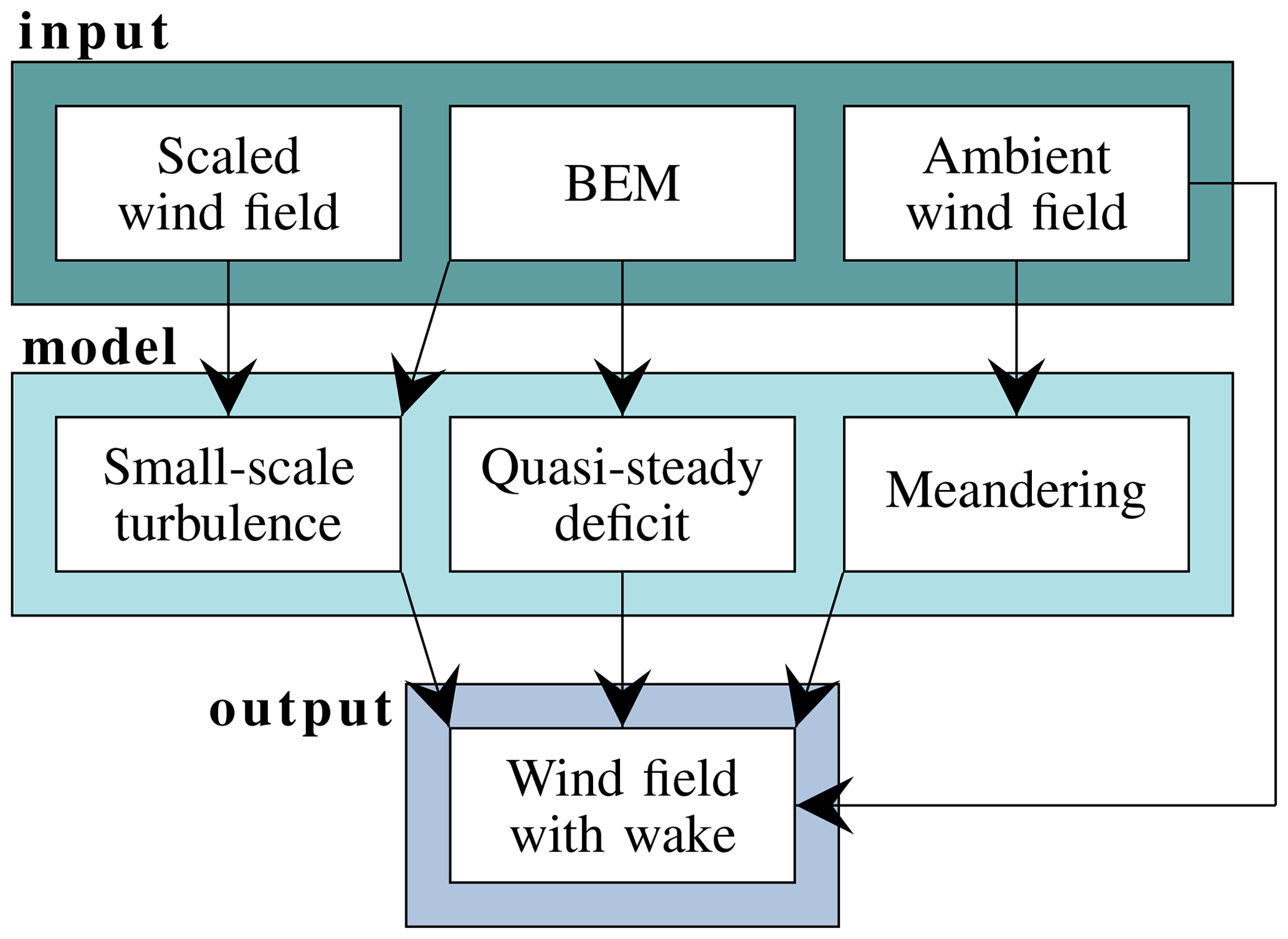
Figure 3Components of the DWM model (adapted from Reinwardt et al., 2018).
The following analysis covers simulated power, blade root flapwise and edgewise bending moments as well as tower bottom bending moments. To compare the measured loads with simulations, sensors at the precise position of the strain gauges are added to the turbine model in alaska/Wind. The locations of the strain gauges are given in Sect. 2.
The measured loads under wake conditions are compared to the simulated loads, which incorporate the DWM model to simulate the inflow at the wake-affected turbine. As mentioned before, the DWM model is based on the assumption that the wake behaves like a passive tracer in the turbulent wind field. Consequently, the movement of the passive structure, i.e., the wake deficit, is driven by large turbulence scales (Larsen et al., 2007, 2008b). The main components of the model are summarized in Fig. 3.
One part of the model is the quasi-steady wake deficit, or rather the wind speed deficit in the MFR, which consists of a definition of the initial deficit emitted by the wake-generating turbine and the degradation of the deficit downstream (Larsen et al., 2008a). The expansion in downstream direction is calculated with the thin shear layer approximation of the Navier–Stokes equations in their axisymmetric form and thus is strongly related to the work of Ainslie (1988). The method in the DWM model is outlined in Larsen et al. (2007). Using a finite-difference method combined with an eddy viscosity (νT) closure approach, the thin shear layer equations are solved directly starting at the rotor plane. The emitted initial deficit serves as a boundary condition when solving the equations. It is based on the axial induction factor derived from the BEM theory. Three calculation methods of the quasi-steady wake deficit, which differ only in the description of the initial deficit and the eddy viscosity, will be compared in the course of this study:
-
“DWM-Egmond” based on the definitions in Madsen et al. (2010) and Larsen et al. (2013),
-
“DWM-Keck-c”, a recalibrated version of the “DWM-Keck” model based on lidar measurements from the wind farm underlying here (Reinwardt et al., 2020).
A detailed description of the individual models can be found in Reinwardt et al. (2020).
Another aspect of the model is the description of the wake meandering. In this work, it is calculated based on the large turbulence scales of the ambient turbulent wind field, which is generated by a Kaimal spectrum and a coherence function (e.g., Veers, 1988) and subsequently ideally low-pass filtered. Afterwards, the vertical and horizontal movements are determined based on the filtered wind field. The cut-off frequency of the low-pass filter is specified by the ambient wind speed and the rotor diameter (Larsen et al., 2013).
The third part of the DWM model is the definition of the small-scale turbulence generated by the wake shear itself as well as by blade tip and root vortices. This small-scale turbulence is calculated with a scaled homogeneous turbulent wind field, which is also generated by a Kaimal spectrum. The scaling is implemented in accordance with IEC 61400-1 Ed.4 (2019). The scaling factor is based on the calculation of the initial deficit, which itself builds on the BEM theory and the aerodynamics of the turbine. A more detailed description of the implementation of the complete model can also be found in Reinwardt et al. (2020).
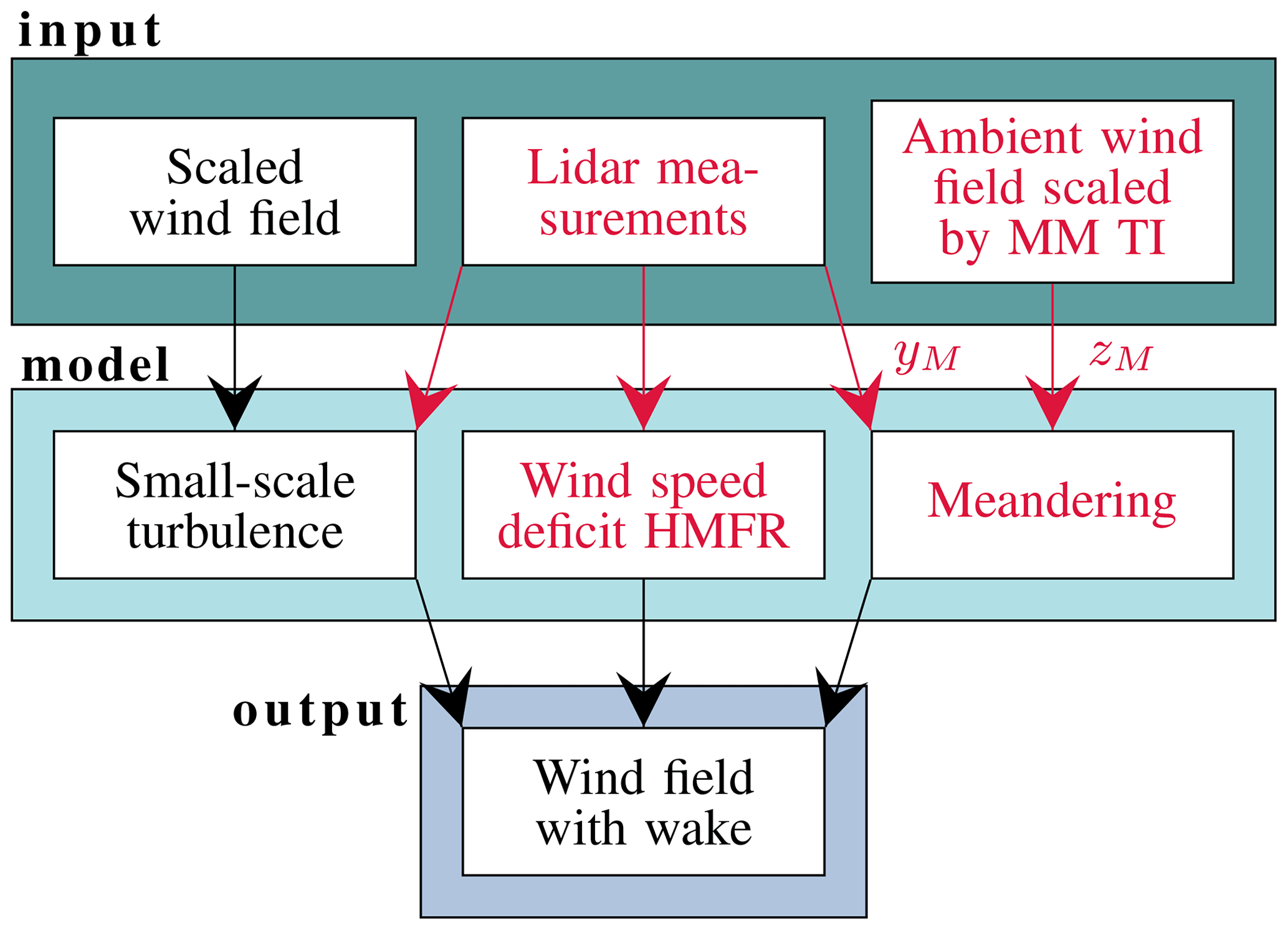
Figure 4Incorporation of lidar measurements into the DWM model; yM is the horizontal and zM the vertical meandering component.
In the previous section, a recalibrated version of the DWM model has been introduced. The lidar systems have been used to recalibrate the DWM model to decrease the uncertainties of load simulations in wake conditions. In a next step, the lidar measurements will be successively incorporated into the wake simulation. A schematic illustration of the process is illustrated in Fig. 4. Firstly, the lidar-measured mean wind speed deficit is used to replace the quasi-steady deficit in the DWM model definition (see also Fig. 3). Since only a horizontal line is scanned, no vertical meandering can be captured (see Sect. 3). To clarify that only the horizontal meandering can be measured and that the transformed wind speed deficit in the MFR is still affected by vertical meandering, because due to the scanning pattern vertical meandering cannot be captured, the phrasing “horizontal meandering frame of reference” (HMFR) is introduced in Fig. 4. In a second step, the measured horizontal meandering is included in the DWM model and the vertical meandering is neglected. The vertical meandering has only a marginal influence on the shape of the deficit in the MFR as explained in Reinwardt et al. (2020).
The lidar system measures in the induction zone of the downstream turbine, where the wind speed is decreased due to the upstream effect of the subsequent turbine. However, its influence must be excluded from the measurement results to use the measured wind speed deficit in the wake model. The simple induction model defined in Troldborg and Meyer Forsting (2017) is applied to account for this effect. The two-dimensional model defines the wind speed in the induction zone as follows:
where is the positive upwind distance normalized by the rotor radius, a0 is the induction factor at the rotor center area defined as , , is the radial distance from the hub normalized by the rotor radius, ct is the thrust coefficient, γ=1.1, , , λ=0.587, and η=1.32. The model has already been used to correct lidar measurements in the induction zone by Dimitrov et al. (2019) and Conti et al. (2020).
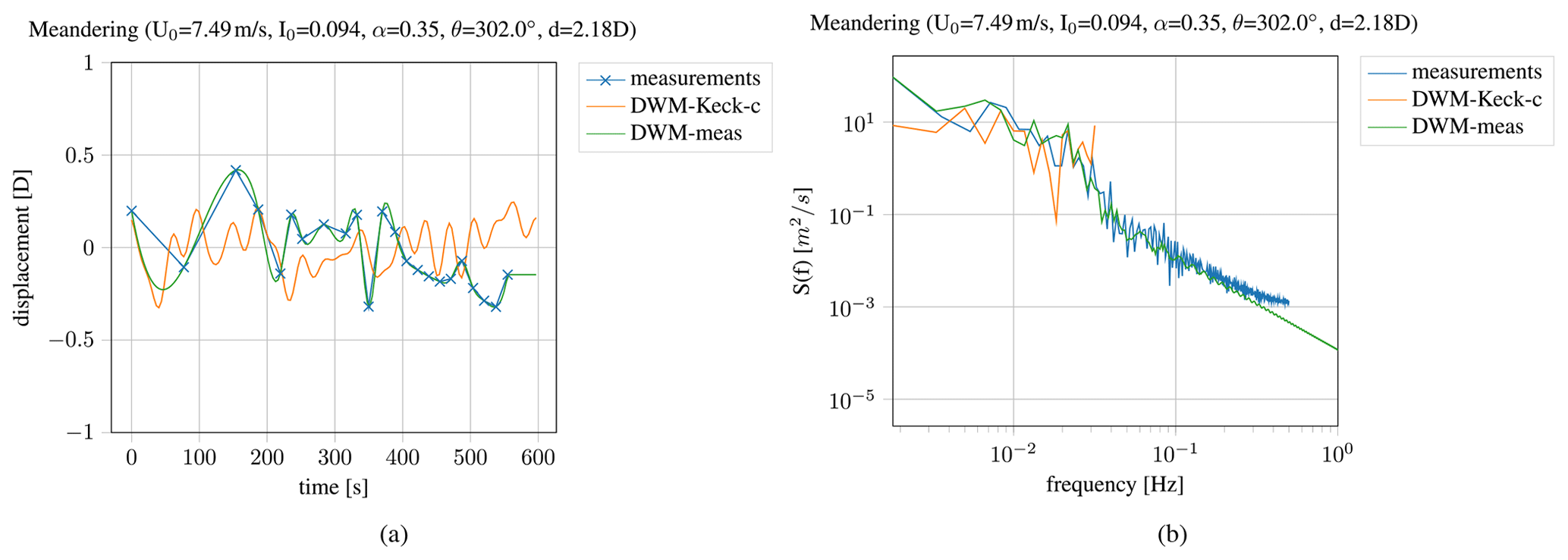
Figure 5Time series (a) and power spectrum (b) of the meandering, measured and simulated with the calibrated DWM-Keck-c model as well as the interpolated time series (DWM-meas).
The time series of the meandering and the horizontal displacement of the wake are determined with the help of a Gaussian fit in accordance with Trujillo et al. (2011), who assume that the probability of the wake position in vertical and horizontal directions is completely uncorrelated. The Gaussian function has been fitted to the wind speed deficit so that the center of the wake could be determined in accordance with the fitting parameters. Since the vertical meandering is neglected in the present case, the measurement results are fitted to a one-dimensional Gaussian curve:
where A1D is a scaling parameter, σy describes the wind speed deficit width, and μy is the horizontal displacement. Determining the measured mean wind speed deficit in the HMFR can be summarized as follows:
-
correction of the measured wind speed by the induction zone model;
-
fitting of a Gaussian curve to the wind speed distribution along the horizontal direction determined by a measured horizontal line scan and determination of the horizontal displacement of the wake;
-
transfer of the measured wind speed deficit to the HMFR by shifting the scan points according to the determined displacement;
-
interpolation of the scanned wind speed deficit in the HMFR to a regular grid;
-
repetition of steps 1 to 4 until a certain number of scans is reached (e.g., approximately 37 for a 10 min time series);
-
calculation of the mean wind speed deficit in the HMFR from all scans; and
-
fitting of the measured mean wind speed deficit to the Bastankhah wake model described in Bastankhah and Porté-Agel (2014).
It should be pointed out that always the closest available measured range gate, which is still outside the rotor area of the downstream turbine, is used to determine the inflow wind speed deficit. Furthermore, the fourth step of interpolating the wind speed deficit to a regular grid is mandatory due to the fact that the horizontal displacement differs at each instant in time, and thereupon the measurement points are transmitted to a different location in the HMFR, so the sixth step of calculating a mean wind speed deficit over all scans is only possible after interpolating all scans to the same regular grid. A more detailed explanation of calculating the wind speed deficit in the HMFR can be found in Reinwardt et al. (2020).

Figure 6Wind speed deficit in the HMFR, measured and simulated with the calibrated DWM-Keck-c model as well as fitted to a Gaussian-shaped wake model (DWM-meas).
An example of the measured and simulated time series of the meandering as well as the power spectrum is shown in Fig. 5. It depicts the measured time series of the meandering as well as the one simulated with the Keck-c model and a random turbulence seed. To incorporate the time series of the meandering in the wake and load simulations, the time series has been cubically interpolated so that a smooth meandering could be included in the wake model and the turbine loads are not increased by an immediate change of the position of the wind speed deficit. The interpolated time series of the meandering is denoted as DWM-meas. The comparison of simulations and measurements shows that the amplitude of the measured time series is slightly more pronounced. Furthermore, at the low-frequency part, the energy content from the measurements is higher. A reason could be that the meandering is modeled based on the ambient wind speed although the wind speed in the wake is reduced. Applying a reduced mean wake wind speed in the meandering calculation procedure would lead to a higher deflection of the wake. It should also be pointed out that the measurement frequency is very low due to the data filtering in the beginning, so it might be the case that some parts of the meandering could not be captured by the measurements.
An example of a measured wind speed deficit over the radial distance from the hub center in the HMFR in comparison to the simulated one with the recalibrated DWM model is illustrated in Fig. 6. The ambient conditions (ambient wind speed U0, ambient turbulence intensity I0, wind shear α and wind direction θ) are defined in the title of the figure. The edges of the measured deficit are coarser than the area close to the center of the deficit. The explanation for this observation is as follows. The distribution generated by the meandering process provides many scan points around the center of the wind speed deficit and only a few at the tails, so the influence of turbulence at the tails is much higher. Thus, the measured wind speed deficit shows a coarse distribution at the boundaries of the deficit. Using this coarse curve and replacing the wind speed deficit description in the DWM model directly by the measured one leads to increased loads in the simulation, which are not feasible; wherefore, the measured wind speed deficit has to be fitted to a smooth curve before applying it in load simulations. Furthermore, the lidar system only measures an opening angle of −20 to 20∘. Hence, particularly for short distances, the deficit is not captured exhaustively. Even the ambient wind speed is not reached at the edges of the curve; thus, it is necessary to extrapolate the wind speed to smoothly meet the ambient wind speed. As a result of these issues, the measured deficit has been fitted to a simple Gaussian-shaped wake model (Bastankhah model) outlined in Bastankhah and Porté-Agel (2014). According to the model, the wind speed deficit can be defined as
with k* being the wake growth rate, the downstream distance normalized by the rotor radius, the normalized hub height, and the normalized horizontal and vertical distance and
The wake growth rate k* has been adjusted to fit the model to the measured deficit in the HMFR. The fitted model is labeled “DWM-meas” in Fig. 6.
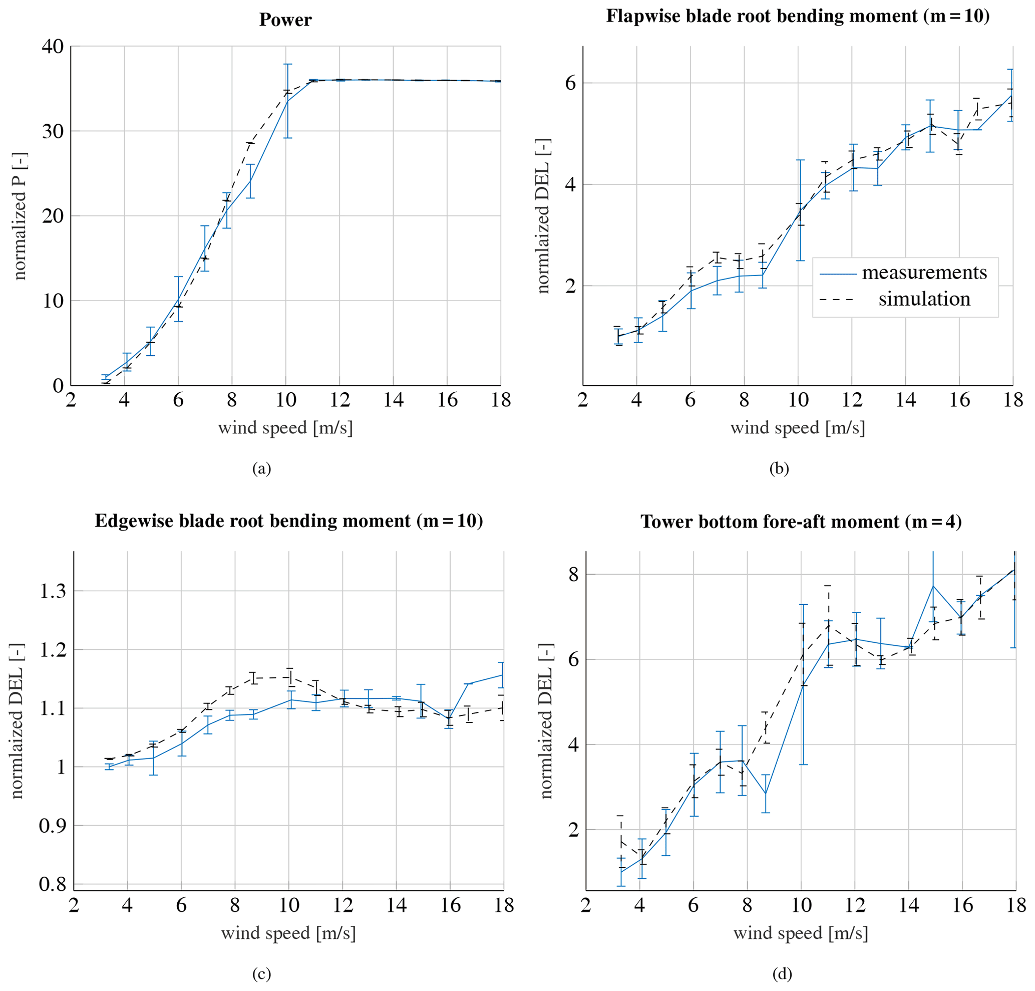
Figure 7Measured and simulated power (a), flapwise blade root moment (b), edgewise blade root moment (c) and tower bottom fore-aft moment (d) at WTG 2 at an ambient turbulence intensity of 12 % and wake-free inflow.
7.1 Comparison of measured and simulated loads and power under wake-free inflow
In order to validate the aerodynamic load simulations, the following section contains a comparison of measured and simulated loads under wake-free inflow conditions. The section shows results from WTG 2 under normal operating conditions. The met mast as well as WTG 2 are exposed to wake-free inflow conditions. Thus, the met mast is suitable to determine all ambient conditions. The mean value of the measured and simulated normalized power curve is depicted in Fig. 7a for a turbulence intensity of 12 %.
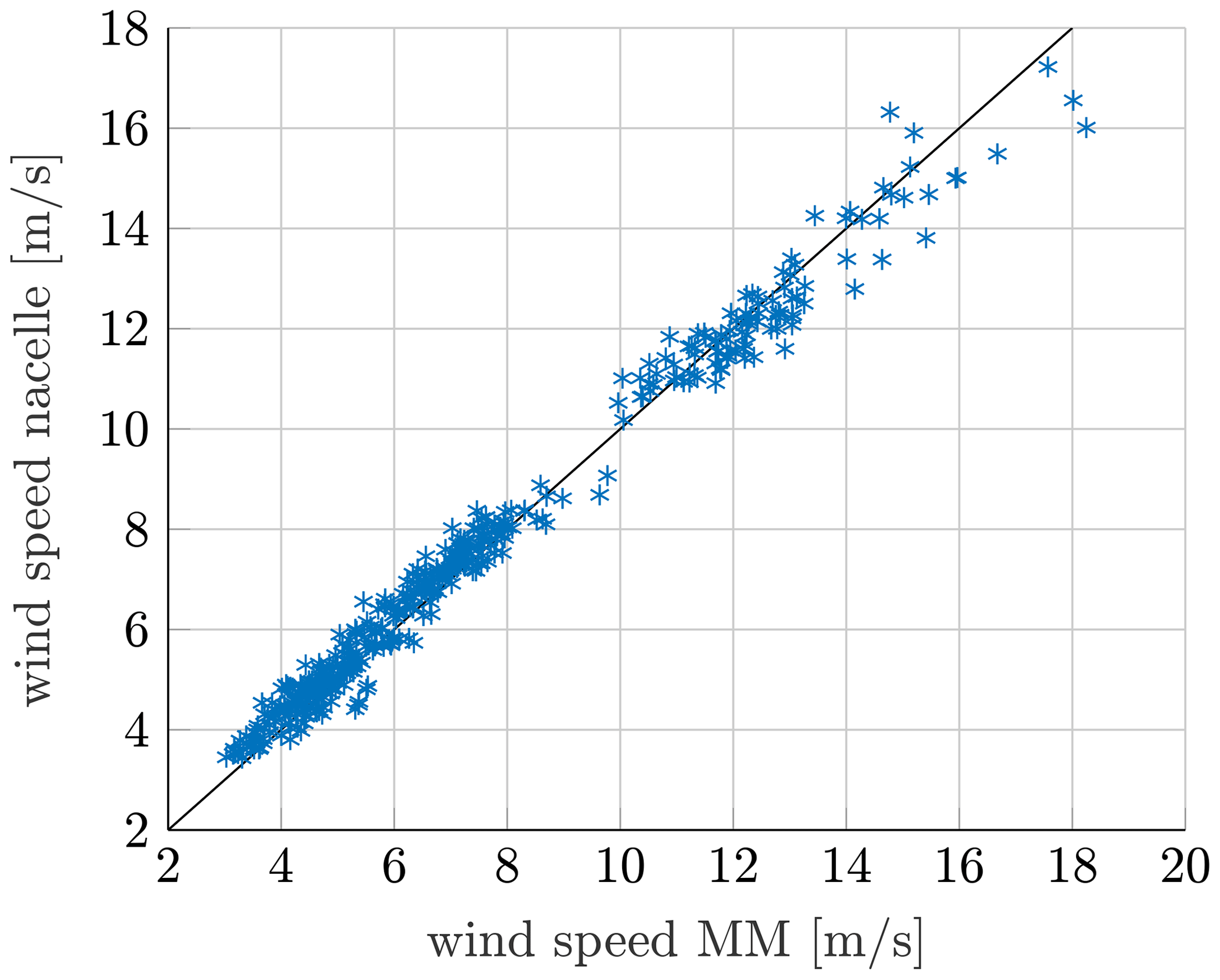
The power curve is normalized by the measured power in the smallest wind speed bin. The error bars in the curves illustrate the standard deviation in each wind speed bin. All data sets are divided into wind speed bins with a width of 1 m s−1. The mean values of wind speed, turbulence intensity, wind shear and air density of each wind speed bin determine the input parameters for the load simulations. Each simulation is conducted six times with different seeds, so the simulation results are likewise shown as mean values with standard deviations. In summary, the simulated power agrees very well with the measured power; solely close to the rated wind speed of 11 m s−1, some discrepancies between measurements and simulations occur. In this area, only a few measurement points can be extracted due to the chosen filtering criteria. As a result, the measurements show an extraordinarily high standard deviation. A comparative study of the measured wind speed of the nacelle anemometer and the met mast has indicated some discrepancies in this range (see Fig. 8). Thus, it is very likely that the deviation arises due to a momentarily different inflow wind speed at the turbine than the one measured at the met mast and used in the simulations. The measured wind speed at the nacelle anemometers is corrected by a nacelle transfer function so that the current inflow wind speed at the turbine can be estimated.
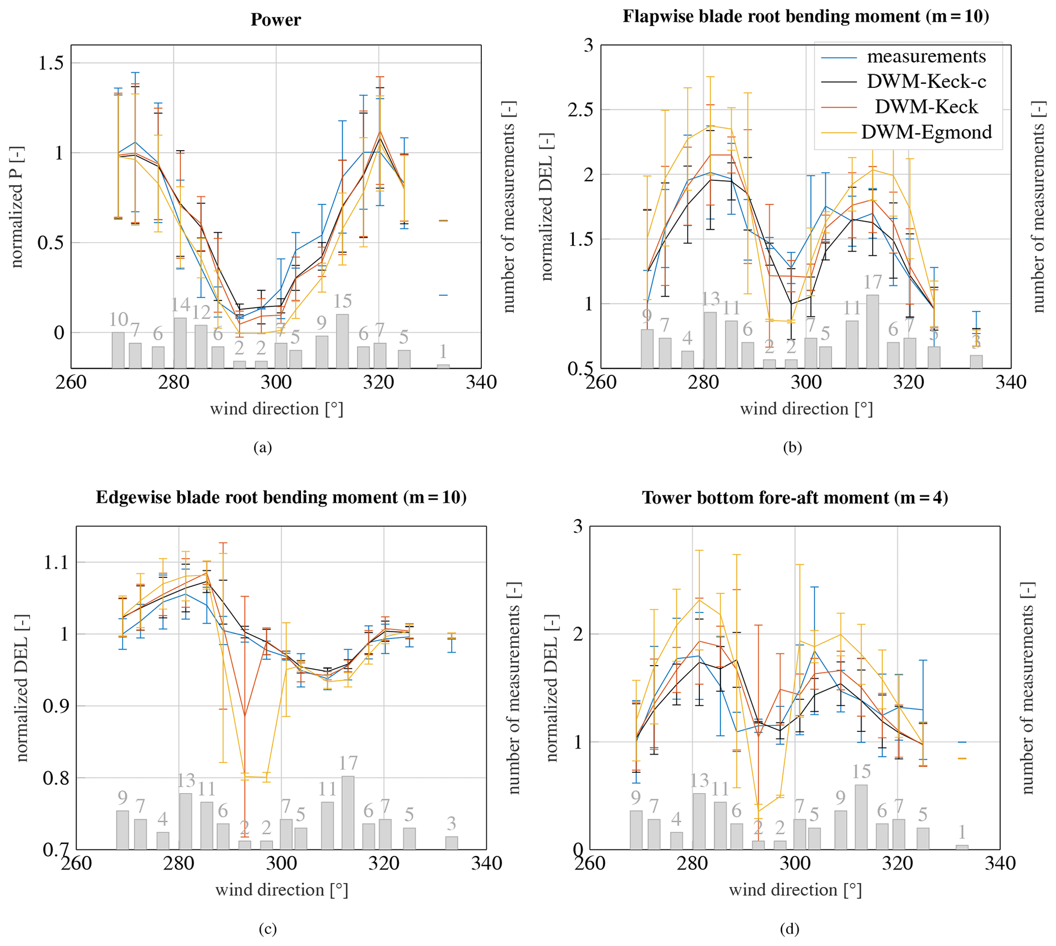
Figure 9Measured and simulated power deficit (a), flapwise blade root moment (b), edgewise blade root moment (c) and tower bottom fore-aft moment (d) at WTG 2 at an ambient wind speed of 6 m s−1 and an ambient turbulence intensity of 6 %. WTG 2 is exposed to the wake of WTG 1. The number of measured 10 min time series in each wind direction bin is illustrated on the secondary axis.
The results of the measured and simulated flapwise blade root bending moment are illustrated in Fig. 7b. It displays the normalized 1 Hz damage-equivalent load (DEL). The Wöhler coefficient (inverse slope of S–N curve) is given in title of the figure. The development of the measured flapwise fatigue load as a function of the wind speed can be reproduced very well by the simulations. Only some slight discrepancies occur between 6 and 9 m s−1, where the simulation overestimates the loads slightly. These discrepancies are assumed to be related to the inaccuracy of the load simulation software itself. The measured and simulated DEL of the edgewise blade root bending moment is depicted in Fig. 7c. The simulations of the edgewise moment show a local maximum just below the rated wind speed. This observation could not be verified by the measurements. The measured and simulated power deviate in this wind speed range, which can be explained by differences between the nacelle anemometer and the met mast anemometer in the estimated wind speeds. It is most likely that the load discrepancies in this range derive from the same issue. The differences in the edgewise moment and the power around the rated wind speed as well as the illustration of the measured nacelle wind speed and the met mast support the hypothesis that the turbine experiences a local momentarily different inflow wind speed and explain the discrepancies. Furthermore, due to the low amount of data points in this region, the measured wind speed might be biased. However, since the differences between measurements and simulations in the edgewise moment are still below 5 %, the overall agreement is reasonable for this load component. The edgewise moment is mainly driven by the rotational speed of the rotor and the gravity. The dependency of the edgewise moment on the wind speed is less pronounced in comparison to the flapwise moment. The simulated DELs of the tower bottom bending moment are depicted in Fig. 7d. The measured tower bottom bending moment can be predicted very well by the simulation, although there are similar discrepancies around the rated wind speed. Nevertheless, the accuracy of the used load simulation software in combination with the turbine model for load simulations is presumed to be appropriate for a further analysis of the wake sectors, since for the wake analysis only results below the rated wind speed are analyzed.
7.2 Comparison of measured and simulated loads and power under wake conditions
7.2.1 Analysis at an ambient wind speed of 6 m s−1 and a turbulence intensity of 6 %
The following section summarizes the measured and simulated fatigue loads under normal operation conditions for the wake sector. The ambient conditions for the simulations are determined by the met mast so that only results with wake-free inflow at the met mast are included in the evaluation. The results of the measured and simulated normalized power deficit, where WTG 2 experiences the wake of WTG 1, are shown in Fig. 9a.
The results are normalized by the measured power at wake-free inflow on the left side of the power deficit curve. The measurements were gathered during an ambient wind speed of 6 m s−1 and an ambient turbulence intensity of 6 %. The number of measured 10 min time series in each wind direction bin is illustrated in the bar graph. The mean values and their corresponding standard deviations are illustrated for each wind direction bin, along with the number of considered measurements and simulations. Close to full wake, only a few measurement points could be collected, whereas towards the edges of the deficit more points could be gathered. The reason is that the deficit towards full wake is very pronounced, and thus the inflow wind speed at the wake-affected turbine is often below the cut-in wind speed. Three different versions of the DWM model are used in the simulations as introduced in Sect. 5. All simulated power deficits agree very well with the measured deficit. There is a slight overestimation of the power deficit calculated by the DWM-Egmond model. Its predicted deficit is so pronounced that in full wake conditions the turbine often does not operate in the simulations. There is a slight decrease of the power above 320∘, which marks the beginning of the wake of WTG 4.
The DELs of the flapwise blade root bending moment under wake conditions are illustrated in Fig. 9b. The Wöhler coefficient is given in title of the figure. The flapwise fatigue loads agree very well with the measurements when using the DWM-Keck-c and DWM-Keck models so that even the two maxima at partial wake conditions are in close agreement. The DWM-Egmond model overpredicts the loads especially at partial wake conditions. At partial wake, the wind speed deficit only affects a section of the rotor, so in combination with the meandering and the horizontal shear of the wind speed, the blade experiences a highly alternating load at each rotation.
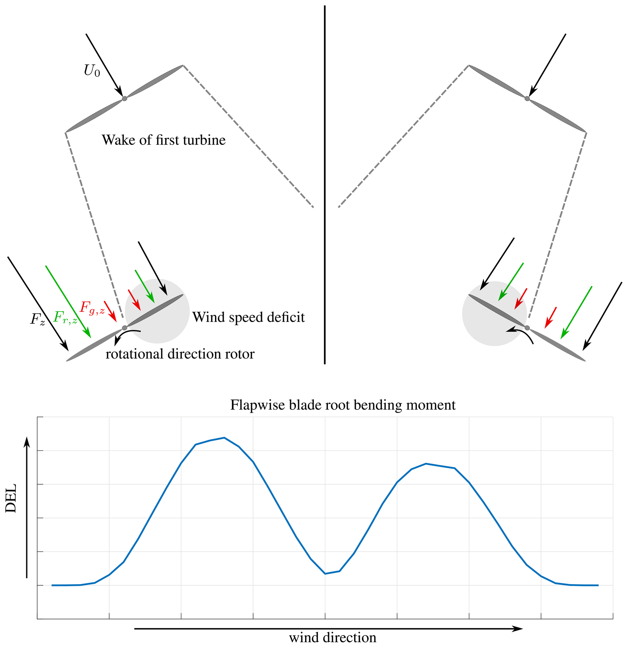
The two maxima are differently pronounced, which derives from the aerodynamic force and the rotor tilt. The aerodynamic forces on a blade segment are a function of the apparent wind velocity, which is a vector composed of the motion of the blade and the incoming wind. Due to the turbine tilt, the apparent wind velocity is slightly lower during the upward movement, and the aerodynamic force is reduced. The blade faces slightly away from the wind direction during the upward movement, whereas during the downward movement, the blade faces slightly more towards the wind direction, which results in an increase of the aerodynamic force. At wake conditions, the increase is stronger when the wind speed deficit coincides with the upward movement of the rotor, so a higher alternating load at the blade occurs and the maximum is more pronounced in comparison to the case where the wind speed coincides with the downwind movement of the rotor. A schematic illustration of phenomenon is depicted in the Appendix in Fig. A1 in order to explain this behavior.
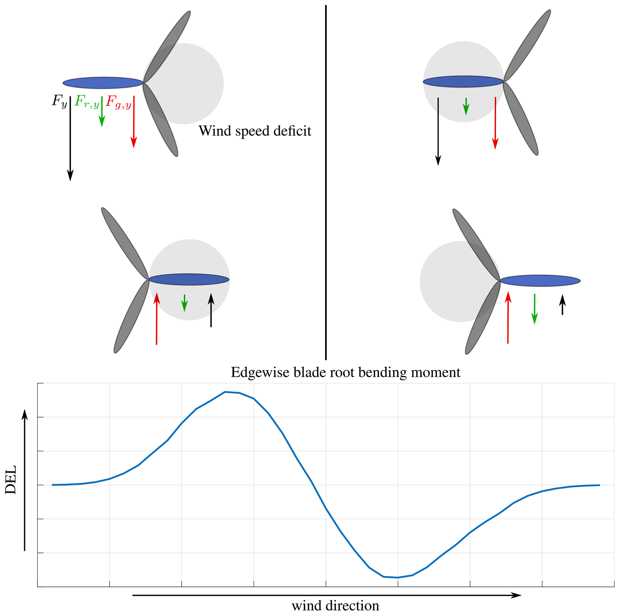
The results of the edgewise blade root bending moment are depicted in Fig. 9c. All models agree similarly well with the measurements. The edgewise moment depends significantly on the blade weight force, while the wake only has a marginal impact on the loads, so the highest increase of the edgewise moment in comparison to wake-free inflow is merely around 5 %. Towards full wake, several outliers in the DWM-Keck and DWM-Egmond model can be recognized. These are related to the simulations, where the turbine does not operate as a result of the low wake wind speed predicted by the models. The rotation of the rotor largely influences the alternating load at the edgewise moment; hence, the fatigue load is drastically reduced when the turbine turns off. The simulations as well as the measurements show an increase of the load in comparison to the wake-free inflow at around 280∘ and even a decrease of the load at around 310∘. The influence of the wind speed is not only related to the rotational speed of the rotor. There is an additional influence due to the tilt of the rotor. The load is defined in the rotating frame of reference so that the weight force switches its sign with each rotation, whereas the influence of the aerodynamic force on the edgewise moment does not change the sign. Thus, at one side of the rotor, the forces level each other out, while on the other side of the rotor they accumulate. If the deficit is on the side, where the forces level each other out, the alternating load increases in comparison to a situation without wake, whereas when the wind speed deficit is on the side, where both aerodynamic and weight force are facing in the same direction, the alternating load is decreased. To clarify this explanation, a schematic illustration is provided in the Appendix in Fig. A2.
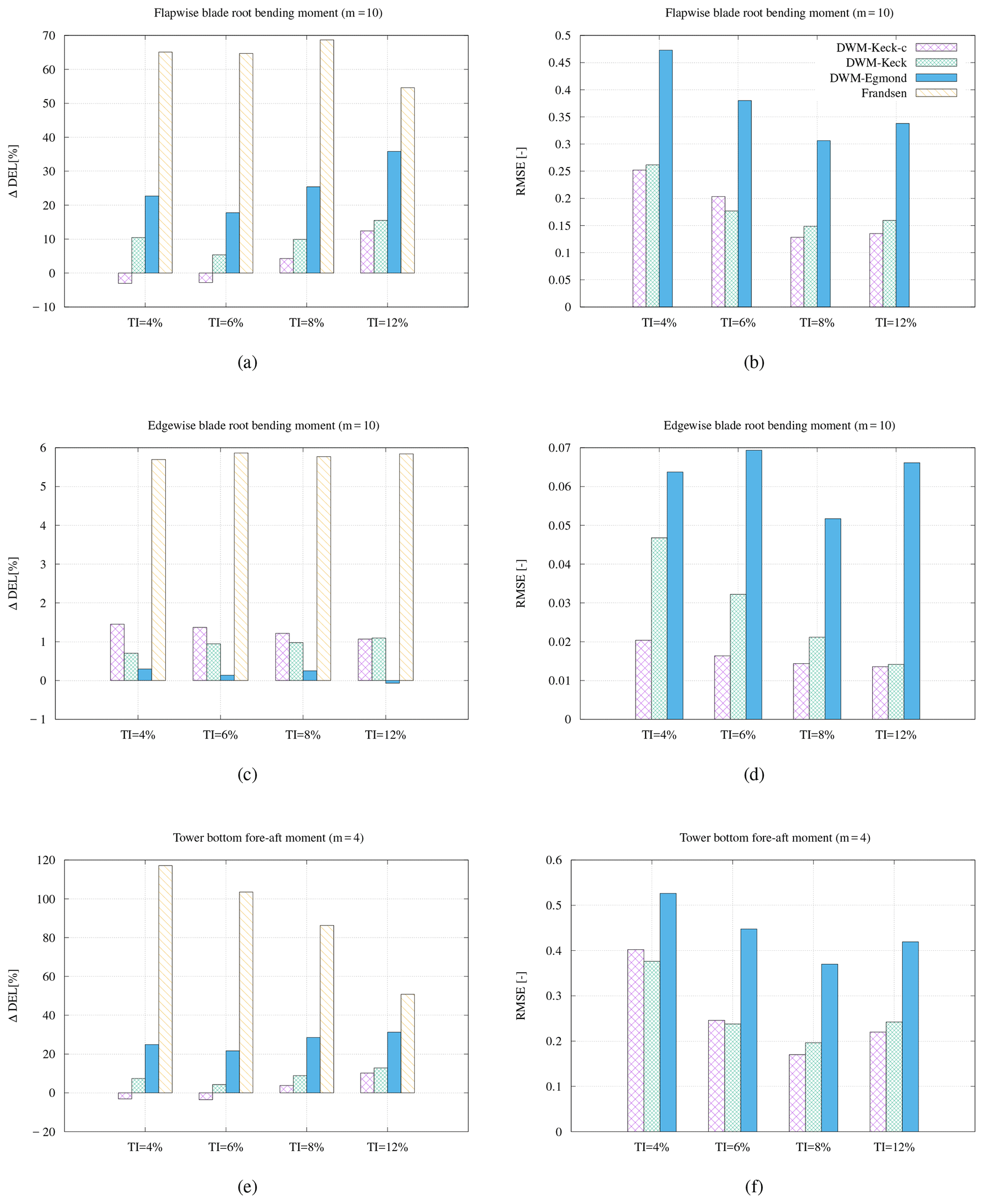
Figure 10Bias between the measured and simulated fatigue loads and the root-mean-square error for the flapwise blade root bending moment (a, b), the edgewise blade root bending moment (c, d) as well as the tower bottom bending moment (e, f) at an ambient wind speed of 6 m s−1. WTG 2 is exposed to the wake of WTG 1.
The tower bottom bending moment is illustrated in Fig. 9d. The two maxima at partial wake conditions that derive from the higher alternating load observed in Fig. 9b are clearly visible for the tower bottom bending moment, too. At full wake conditions, the load is only slightly increased in comparison to wake-free inflow. Though, similar to the flapwise moment, the tower bottom bending moment is almost doubled at partial wake conditions. The results of all three models agree well with the measurements. Only the DWM-Egmond model overestimates the loads, as it could already be seen in the blade flapwise and edgewise moments.
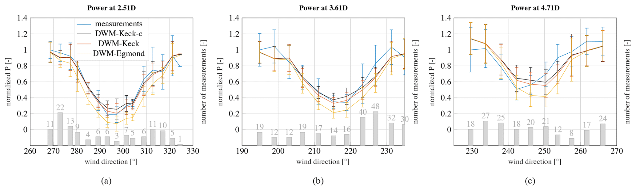
Figure 11Measured and simulated power at an ambient wind speed of 8 m s−1 and an ambient turbulence intensity of 10 % when WTG 2 is exposed to the wake of WTG 1 (a), WTG 5 is exposed to the wake of WTG 2 (b), and WTG 5 is exposed to the wake of WTG 1 (c). The number of measured 10 min time series in each wind direction bin is illustrated on the secondary axis.
7.2.2 Comparison of different turbulence intensities
A similar analysis as the one presented in Fig. 9 is carried out for different turbulence intensity bins and summarized in Fig. 10. A comparison of the results of the flapwise bending moment over all turbulence intensity bins is shown in Fig. 10a. It illustrates the bias of the accumulated DEL over all wind directions. A negative value implies a lower value of the simulated accumulated DEL than the measured DEL. The accumulated DEL over all wind directions is calculated with respect to the Wöhler coefficient. A Wöhler coefficient of 10 is used for the blades and 4 for the tower loads as specified in the titles. Of all models, the recalibrated DWM-Keck-c model coincides best with the measurements over all turbulence intensity bins. At small turbulence intensities, the DWM-Keck-c model underestimates the accumulated DEL slightly. The DWM-Egmond model overestimates the accumulated DEL drastically, especially at high turbulence intensities. The root-mean-square error (RMSE) of the flapwise bending moment between the simulation and the measurement over the wind directions is given in Fig. 10(b). The RMSEs of the DWM-Keck and the recalibrated DWM-Keck-c model are very similar, while the DWM-Egmond delivers the highest RMSE. The reason for illustrating the deviation between measurements and simulations ΔDEL as well as the RMSE is that the deviation of the accumulated DEL expresses how accurate the models perform in a site-specific load calculation procedure. Additionally, it allows a comparison with the Frandsen wake-added turbulence model (Frandsen, 2007), whereas the RMSE represents the overall capability of predicting the distribution of the DEL over the wind direction. Note that the Frandsen model overestimates the DELs significantly throughout all turbulence intensities.
Figure 10c–d depict the accumulated DELs and the RMSE of the edgewise blade root bending moment. The smallest deviation between the accumulated DELs is achieved with the DWM-Egmond model, but the difference between the models is very small, so that even the highest deviation with the DWM-Keck-c model is only about 1.4 %. The RMSE of the DWM-Keck-c model is the lowest (see Fig. 10d). However, it should be pointed out that also the RMSE is very low in all cases. The results over different turbulence intensity bins of the tower bottom fore-aft bending moment are shown in Fig. 10e–f. Similar to the flapwise moment, the accumulated DEL over all wind directions calculated by the DWM-Keck-c model agrees very well with the measurements. Again, only a slight underestimation occurs at small turbulence intensities. The DWM-Egmond as well as the Frandsen wake-added turbulence model overestimate the accumulated DEL substantially. The RMSEs of the recalibrated and the original model are low and have similar magnitudes. The DWM-Egmond model delivers the highest RMSE over all turbulence intensity bins.
7.2.3 Comparison of different downstream distances
This section compares results for different downstream distances at an ambient wind speed of 8 m s−1 and an ambient turbulence intensity of 10 %. The following three wake situations have been analyzed:
-
WTG 2 in the wake of WTG 1
→ turbine distance =2.51D; -
WTG 5 in the wake of WTG 2
→ turbine distance =3.61D; and -
WTG 5 in the wake of WTG 1
→ turbine distance =4.71D.
The results of the power deficit over the wind directions for these three different distances are shown in Fig. 11. The plots display the mean value in each wind direction bin accompanied by the corresponding standard deviation as an error bar. The same DWM model versions as previously discussed are compared. The notation of the models and the basic structure of the plots follow the figures of Sect. 7.2.1. The closest turbine distance of 2.51D shows the most pronounced deficit, and vice versa. The predicted results of all models agree very well with the measurements. The DWM-Egmond model overestimates the deficit, especially at the largest distance of 4.71D.
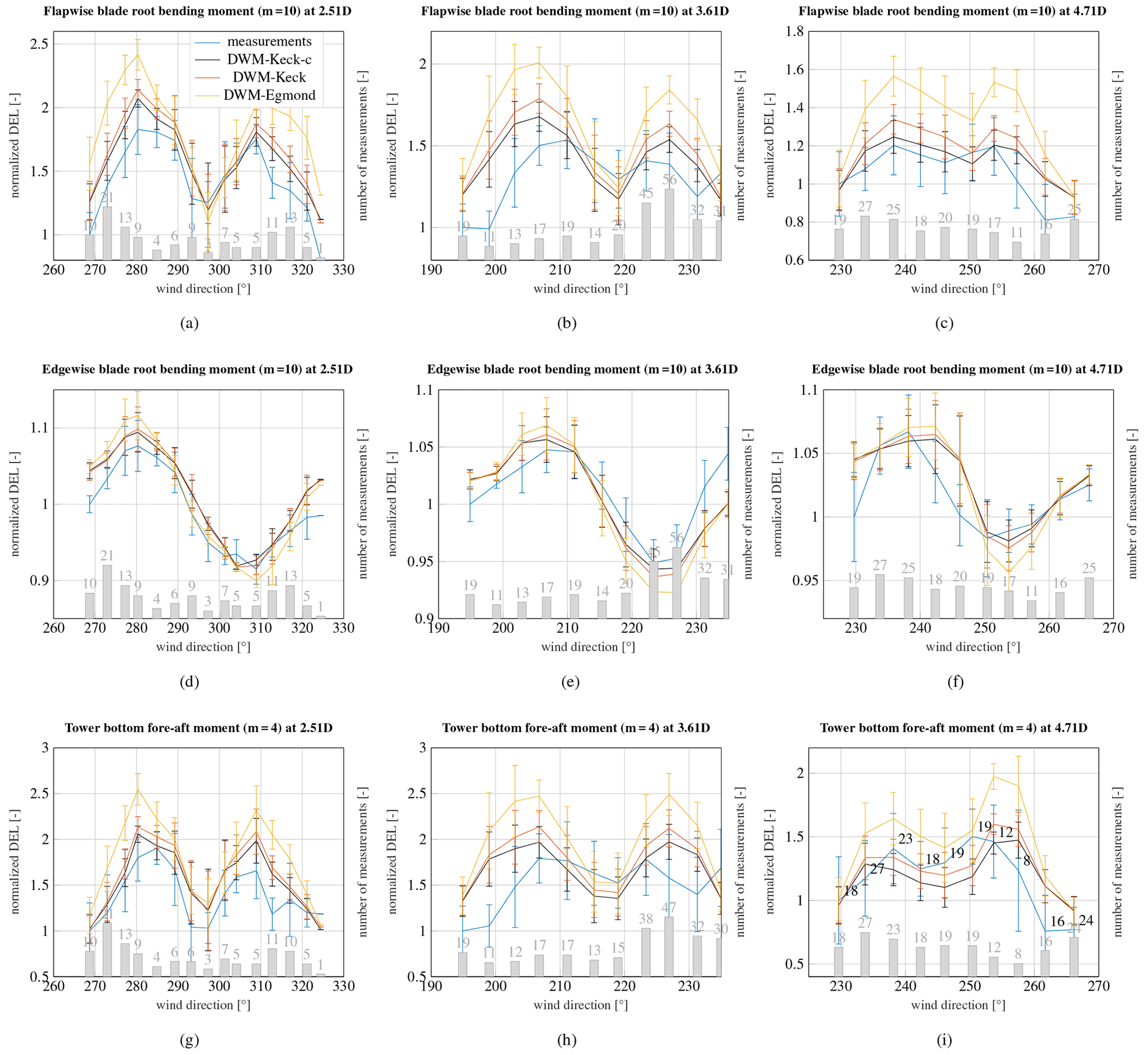
Figure 12Measured and simulated flapwise blade root bending moment (a–c), edgewise blade root bending moment (d–f) and tower bottom bending moment (g–i). WTG 2 is exposed to the wake of WTG 1 in panels (a), (d) and (g), WTG 5 is exposed to the wake of WTG 2 in panels (b), (e) and (h), and WTG 5 is exposed to the wake of WTG 1 in panels (c), (f) and (i). The ambient wind speed is 8 m s−1 and the ambient turbulence intensity is 10 %. The number of measured 10 min time series in each wind direction bin is illustrated on the secondary axis.
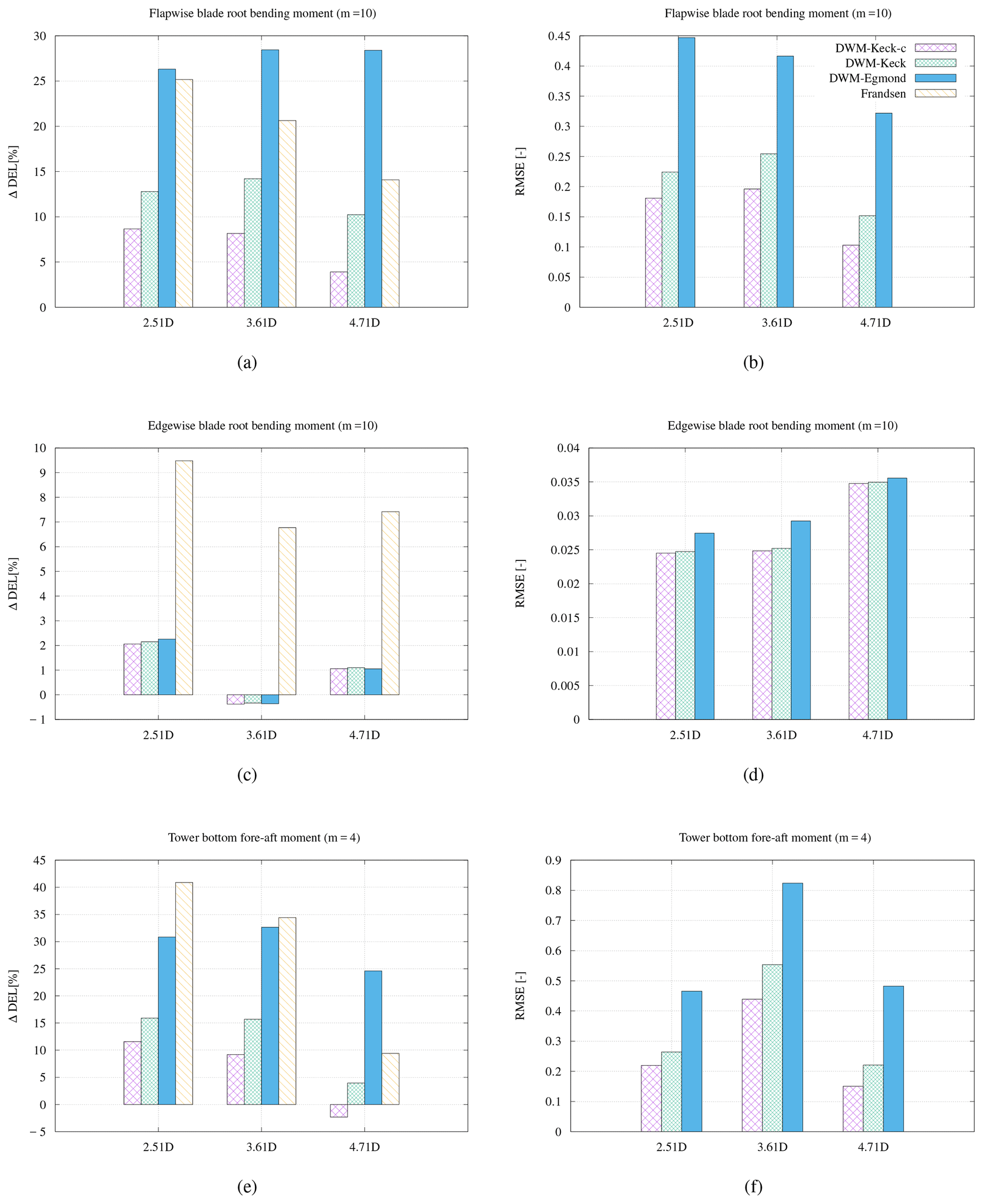
Figure 13Bias between the measured and simulated fatigue loads and the root-mean-square error for the flapwise blade root bending moment (a, b), the edgewise blade root bending moment (c, d), as well as the tower bottom bending moment (e, f) at an ambient wind speed of 8 m s−1 and an ambient turbulence intensity of 10 %.
The results of the flapwise and edgewise blade root moments as well as the tower bottom bending moments are shown in Fig. 12. The results of the recalibrated, and the original DWM-Keck models agree very well with the measurements over all distances. The DWM-Egmond model on the other hand overestimates the loads mostly, particularly at the highest distance of 4.71D. The reason is that the degradation of the wake over the downstream distance is underestimated by this model. The eddy-viscosity definition in the DWM-Keck-c model has been recalibrated by lidar measurements from the site. As a result, a higher and more suitable degradation of the wake could be achieved.
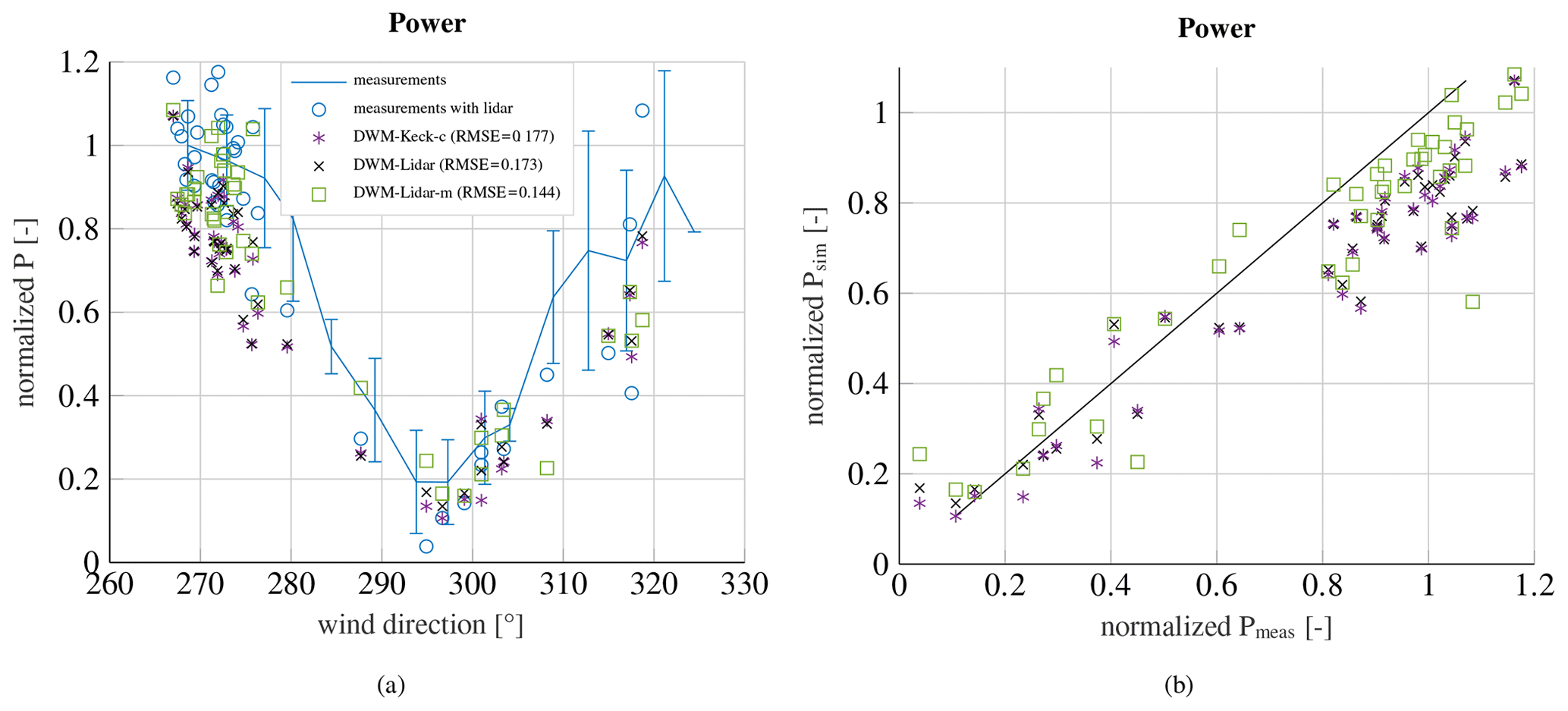
Figure 14Measured and simulated power over the wind direction (a) and simulated power over measured power (b) at an ambient wind speed of 8 m s−1 and an ambient turbulence intensity of 10 %, when WTG 2 is exposed to the wake of WTG 1.
The bias of accumulated DELs over all wind directions as well as the RMSE are depicted in Fig. 13. The recalibrated DWM-Keck model delivers the lowest deviation and RMSE over all distances for the flapwise moment and the tower bottom bending moment, whereas the edgewise blade root bending moment is not improved by the recalibration. However, as mentioned in the previous section, the difference between the results of the single variations of the DWM model is very low for this load component, so all models agree very well with the measurements of the edgewise moment with the exception of the Frandsen wake-added turbulence model. The reason for this is probably that no wind speed deficit is considered in Frandsen's model so that the alternating load at the flapwise moment is higher due to the higher wind speed and the rotational speed of the rotor. The DWM-Egmond model overestimates the loads over all downstream distances. Towards greater downstream distances, the improvement due to the recalibration increases. Lastly, the Frandsen model overestimates the loads over all distances, in particular for close spacings.
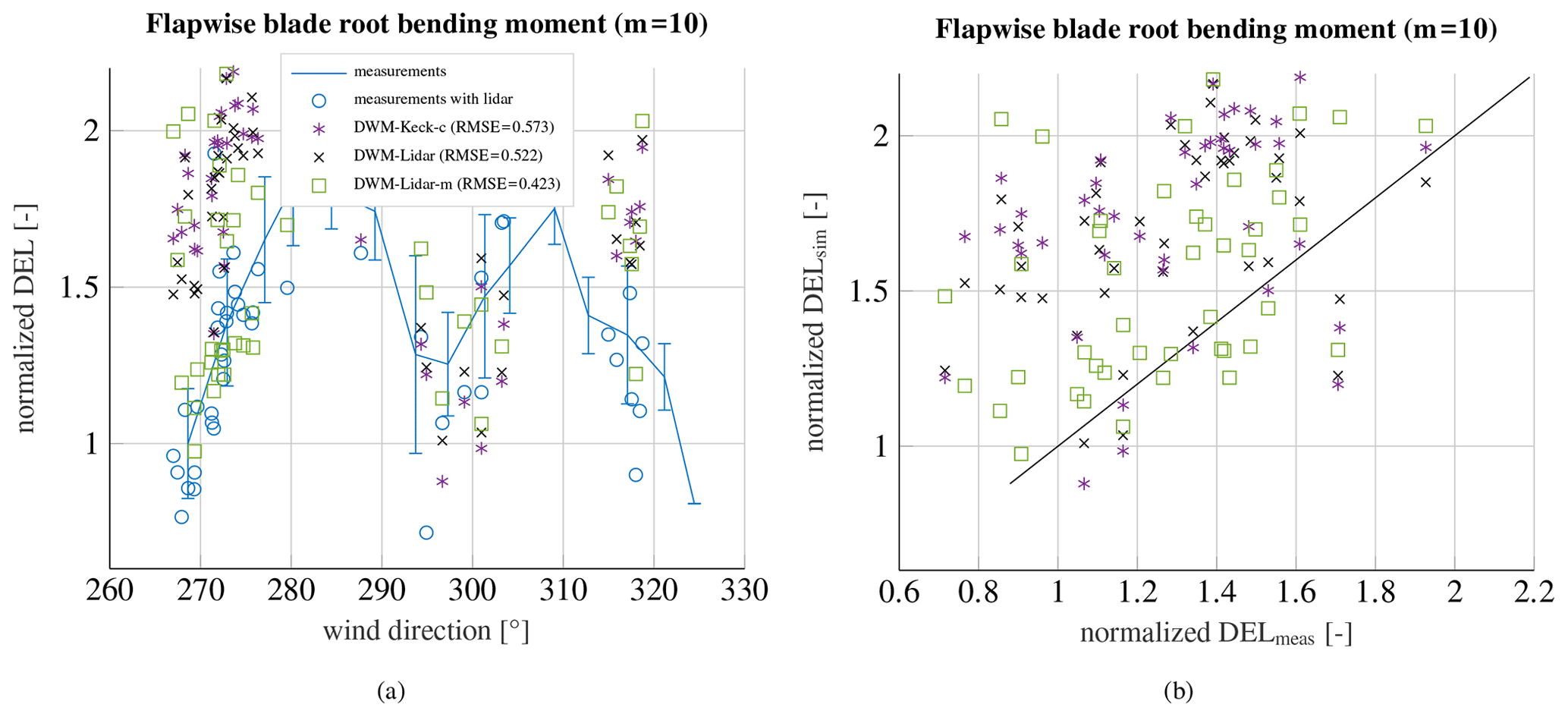
Figure 15Measured and simulated flapwise blade root bending moment over the wind direction (a) and simulated loads over measured loads (b) at an ambient wind speed of 8 m s−1 and an ambient turbulence intensity of 10 %, when WTG 2 is exposed to the wake of WTG 1.
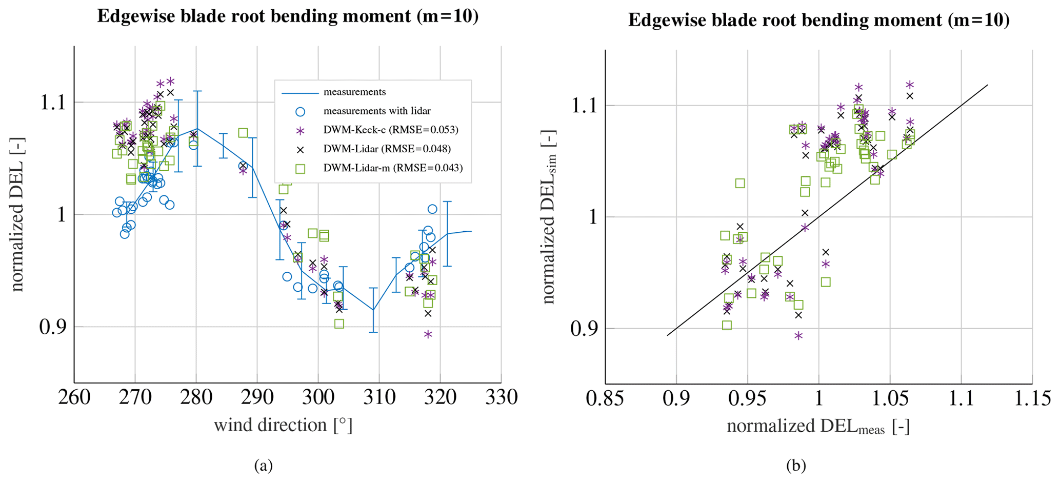
Figure 16Measured and simulated edgewise blade root bending moment over the wind direction (a) and simulated loads over measured loads (b) at an ambient wind speed of 8 m s−1 and an ambient turbulence intensity of 10 %, when WTG 2 is exposed to the wake of WTG 1.
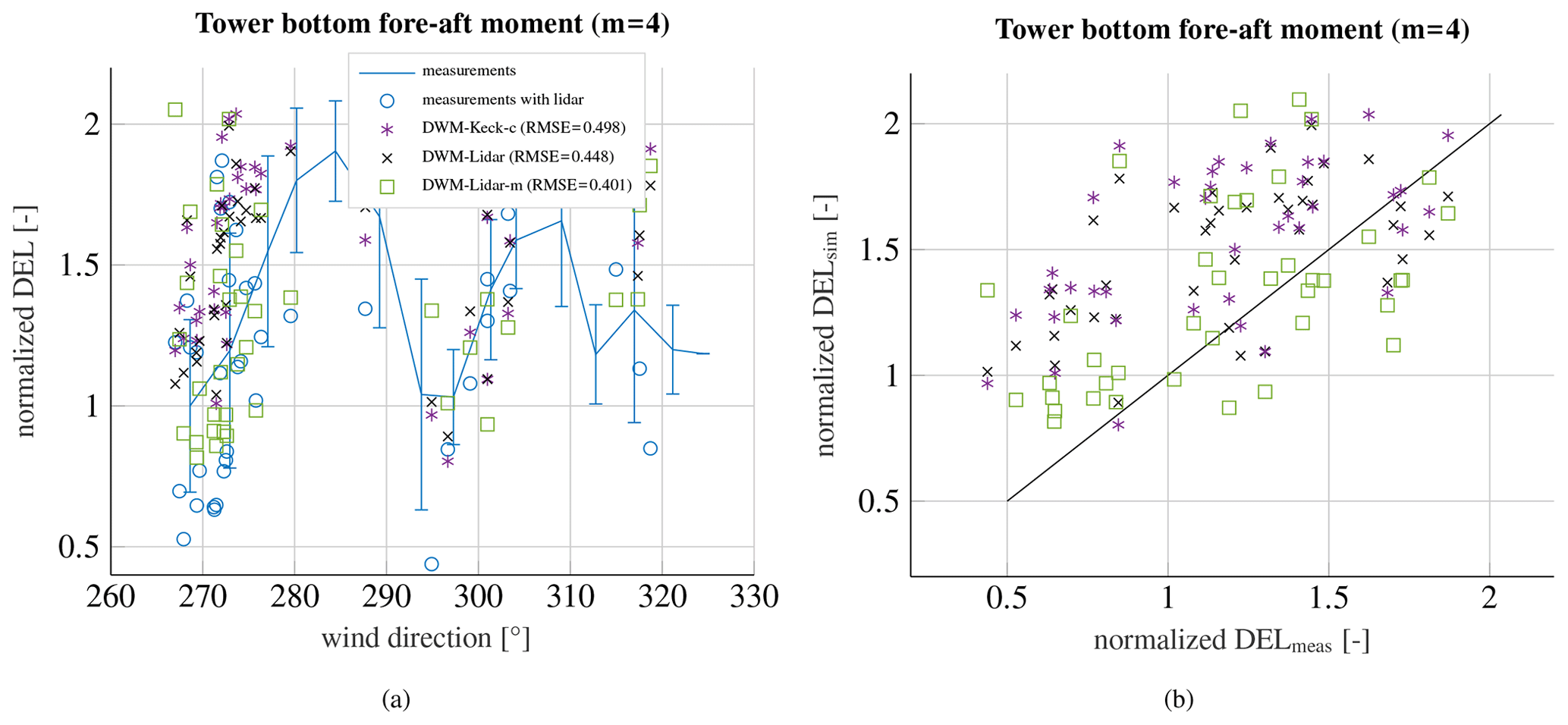
Figure 17Measured and simulated tower bottom fore-aft bending moment over the wind direction (a) and simulated loads over measured loads (b) at an ambient wind speed of 8 m s−1 and an ambient turbulence intensity of 10 %, when WTG 2 is exposed to the wake of WTG 1.
7.2.4 Comparison with lidar-assisted load simulations
In the following, the recalibrated DWM model is compared to a constrained simulation with lidar measurements of the meandering and the wind speed deficit. The method to incorporate the wind speed deficit in the HMFR as well as the meandering itself is explained in Sect. 6. Figure 14a shows the measured power deficit at WTG 2 when the turbine is exposed to the wake of WTG 1 at an ambient wind speed of 8 m s−1 and an ambient turbulence intensity of 10 %. The solid blue curve with error bars is the measured mean power deficit with all measurement results that comply with the requirements for ambient conditions and the filtering criteria. Lidar measurements were not available for all collected data sets. The blue circles illustrate the 10 min time series, where lidar measurements are available. The stars denote the simulated 10 min series using the recalibrated version of the DWM model (DWM-Keck-c). The crosses represent the results when incorporating only the measured wind speed deficit in the HMFR fitted to the Gaussian-shaped wind speed deficit model (DWM-Lidar), whereas the squares consider both the measured meandering and the wind speed deficit in the HMFR (DWM-Lidar-m). The RMSEs between measurements (blue circles) and simulations are given in the legend. The recalibrated DWM model and the constrained simulations, which only use the measured wind speed deficit shape, agree similarly well with the measurements, but the results based on the incorporation of the measured meandering (DWM-Lidar-m) fit considerably better to the measurements, especially towards the left part of the curve. It has been observed that the meandering is more pronounced in the measurements than in the DWM model simulations as it could already be seen in Fig. 5. Thus, especially at the edges of the wake, when the downstream turbine is almost out of the wake, the amplitude of meandering becomes more important. If the meandering is more pronounced in this region, the wake-affected turbine experiences wake-free inflow conditions more often. Furthermore, if there is a slight misalignment of the wake-generating turbine, it is indirectly captured in the determination of the meandering.
The normalized simulated power over the normalized measured power is illustrated in Fig. 14b. The plotted straight black line has a slope of 1 and serves as a reference. The underestimation of the power deficit in the simulations is clearly visible in the upper part of the figure, just like the improvement when considering the measured meandering.
The results of the flapwise blade root bending moment are given in Fig. 15. A clear overestimation of the loads can be seen in the flapwise moment, so there is a higher influence of the wake in the simulations. The incorporation of the wind speed deficit (DWM-Lidar) leads to a slightly better agreement between measurements and simulations than only using the recalibrated DWM model. Including the time series of the meandering (DWM-Lidar-m) leads to even better coincidences between measurements and simulations. However, the simulations overestimate the loads towards the edges of the curve. Similar behavior can be seen for the edgewise moment as well as the tower bottom bending moment (see Figs. 16 and 17), although the difference between simulations and measurements are smaller for these load components. An explanation for the differences and uncertainties can be found in the different downstream distance, which is used in the simulations. For the comparison, measurements at the closest available lidar range gate that is still outside the rotor area of the downstream turbine are used. Thus, it happens that the downstream distance used in the simulations is slightly too low. The lidar specifically measures in 30 m range gates so that no measurements are available at the exact position of the downstream turbine. To achieve a suitable comparison with the DWM-Keck-c model, the measurement distance has been used in the model as well. However, the influence should be rather small due to the small gradient of the wind speed in downstream direction; hence, it does not explain all differences completely. Especially, an overestimation of the power cannot be explained by the too low downstream distance, wherefore it is assumed that some discrepancies are related to a bias in the determination of the ambient conditions and/or the load simulation itself. Furthermore, it should be pointed out that the vertical meandering is neglected, when the measured meandering is used, due to the fact that no vertical meandering is captured by the lidar systems. The vertical movement is less pronounced than the horizontal meandering and has only a small influence on the shape of the wind speed deficit in the fixed frame of reference and the loads. Hence, this simplification barely affects the overall results.
The outlined analysis validates the DWM model based on power and load measurements at an onshore wind farm with small turbine distances. Special focus is put on a calibrated version of the DWM model (Reinwardt et al., 2020). The model has been calibrated based on nacelle-mounted lidar measurements. Additionally, a comparison with the commonly used Frandsen wake-added turbulence model is performed. The newly calibrated model fits very well to measurement results, whereas the Frandsen model delivers very conservative results for small turbine distances. Furthermore, a constrained wake model simulation based on the lidar measurements is presented. The measured wind speed deficit in HMFR as well as the measured time series of the meandering are incorporated into the wake simulations. The incorporation of the wind speed deficit leads to insignificant improvements, which indicates that the shape of the wind speed deficit in the MFR could already be reproduced very well by the recalibrated version. However, only a horizontal line with few scan points has been measured with the lidar system. Thus, a more detailed scan of the wake with a higher temporal resolution might lead to a further decrease of the uncertainties. The incorporation of the time series of the meandering results in a better agreement with the measured power as well as blade root and tower bending moments. All in all, the constrained simulations with lidar measurements verify that the conformity between measured and simulated loads can be enhanced by incorporating the measured meandering as well as the wind speed into the aeroelastic load simulation. This indicates that there is still room for improvements in the physical description of the meandering, the local turbulence and the deficit modeling in the DWM model and confirms in particular the significance of further research on wake meandering.
Access to lidar and met mast data can be requested from the authors.
IR performed all simulations, postprocessed and analyzed the measurement data and wrote the paper. LS monitored the load measurements and data acquisition. Furthermore, LS, DS and ND gave technical advice in regular discussions and reviewed the paper. PD and MB supervised the investigations and reviewed the paper and its revision.
The authors declare that they have no conflict of interest.
The content of this paper was developed within project NEW 4.0 (North German Energy Transition 4.0).
This research has been supported by the Federal Ministry for Economic Affairs and Energy (BMWI) (grant no. 03SIN400).
This paper was edited by Sandrine Aubrun and reviewed by two anonymous referees.
Ainslie, J. F.: Calculating the flowfield in the wake of wind turbines, J. Wind Eng. Ind. Aerodyn., 27, 213–224, 1988. a, b, c
Bastankhah, M. and Porté-Agel, F.: A new analytical model for wind-turbine wakes, Renew. Energ., 70, 116–123, 2014. a, b, c
Burton, T.: Wind energy handbook, Wiley, Berlin, Heidelberg, Germany, 2011. a
Conti, D., Dimitrov, N., and Peña, A.: Aeroelastic load validation in wake conditions using nacelle-mounted lidar measurements, Wind Energ. Sci., 5, 1129–1154, https://doi.org/10.5194/wes-5-1129-2020, 2020. a, b, c
Dimitrov, N., Borraccino, A., Peña, A., Natarajan, A., and Mann, J.: Wind turbine load validation using lidar‐based wind retrievals, Wind Energy, 22, 1512–1533, https://doi.org/10.1002/we.2385, 2019. a, b
Frandsen, S.: Turbulence and turbulence-generated structural loading in wind turbine clusters, PhD thesis, Technical University of Denmark, Roskilde, 130 pp., 2007. a, b
Gerke, N., Reinwardt, I., Dalhoff, P., Dehn, M., and Moser, W.: Validation of turbulence models through SCADA data, J. Phys. Conf. Ser., 1037, 072027, https://doi.org/10.1088/1742-6596/1037/7/072027, 2018. a
IEC 61400-1 Ed.4: IEC 61400-1 Ed. 4: Wind energy generation systems – Part 1: Design requirements, Guideline, International Electrotechnical Commission (IEC), available at: https://standards.iteh.ai/catalog/standards/iec/3454e370-7ef2-468e-a074-7a5c1c6cb693/iec-61400-1-2019 (last access: 18 March 2021), 2019. a, b
IEC 61400-12-1: IEC 61400-12-1: Wind energy generation systems – Part 12-1: Power performance measurements of electricity producing wind turbines, Guideline, International Electrotechnical Commission (IEC), available at: https://standards.iteh.ai/catalog/standards/iec/b6b43db0-b0ba-41a0-baaa-2a027c60cc9b/iec-61400-12-1-2017 (last access: 18 March 2021), 2017. a
Jensen, N. O.: A note on wind generator interaction, Technical Report, Risø-M-2411(EN), Risø, National Laboratory, Roskilde, Denmark, 1983. a
Keck, R.-E.: A consistent turbulence formulation for the dynamic wake meandering model in the atmospheric boundary layer, PhD thesis, Technical University of Denmark, Lyngby, 217 pp., 2013. a
Keck, R.-E.: Validation of the standalone implementation of the dynamic wake meandering model for power production, Wind Energy, 18, 1579–1591, 2015. a
Larsen, G. C.: A simple stationary semi-analytical wake model, Technical Report Risø R-1713(EN), Risø National Laboratory, Roskilde, Denmark, 2009. a
Larsen, G. C., Madsen, H. A., Bingöl, F., Mann, J., Ott, S., Sørensen, J. N., Okulov, V., Troldborg, N., Nielsen, M., Thomsen, K., Larsen, T. J., and Mikkelsen, R.: Dynamic wake meandering modeling, Technical Report Risø-R-1607(EN), Risø National Laboratory, Roskilde, Denmark, 2007. a, b
Larsen, G. C., Madsen, H. A., Larsen, T. J., and Troldborg, N.: Wake modeling and simulation, Technical Report Risø-R-1653(EN), Risø National Laboratory, Roskilde, Denmark, 2008a. a
Larsen, G. C., Madsen, H. A., Thomsen, K., and Larsen, T. J.: Wake meandering: A pragmatic approach, Wind Energy, 11, 377–395, https://doi.org/10.1002/we.267, 2008b. a, b
Larsen, T. J., Madsen, H. A., Larsen, G. C., and Hansen, K. S.: Validation of the dynamic wake meander model for loads and power production in the Egmond aan Zee wind farm, Wind Energy, 16, 605–624, 2013. a, b, c
Machefaux, E., Troldborg, N., Larsen, G., Mann, J., and Aagaard Madsen, H.: Experimental and numerical study of wake to wake interaction in wind farms, in: Proceedings of the European Wind Energy Conference and Exhibition (EWEA 2012), Copenhagen, Denmark, 16 Monday–Thursday 19 April 2012, 10 pp., 2012. a
Madsen, H. A., Larsen, G. C., Larsen, T. J., and Troldborg, N.: Calibration and validation of the dynamic wake meandering model for implementation in an aeroelastic code, J. Sol. Energy Eng., 132, 041014, https://doi.org/10.1115/1.4002555, 2010. a, b
Quarton, D. C. and Ainslie, J.: Turbulence in wind turbine wakes, Wind Engineering, 14, 15–23, 1989. a
Reinwardt, I.: Vergleich und Untersuchung der Auswirkung von Nachlaufmodellen auf Betriebslasten und Leistung von Windenergieanlagen, Master thesis, HAW Hamburg, Hamburg, Germany, 170 pp., 2017. a, b
Reinwardt, I., Gerke, N., Dalhoff, P., Steudel, D., and Moser, W.: Validation of wind turbine wake models with focus on the dynamic wake meandering model, J. Phys. Conf. Ser, 1037, 072028, https://doi.org/10.1088/1742-6596/1037/7/072028, 2018. a, b, c
Reinwardt, I., Schilling, L., Dalhoff, P., Steudel, D., and Breuer, M.: Dynamic wake meandering model calibration using nacelle-mounted lidar systems, Wind Energ. Sci., 5, 775–792, https://doi.org/10.5194/wes-5-775-2020, 2020. a, b, c, d, e, f, g, h, i
Troldborg, N. and Meyer Forsting, A. R.: A simple model of the wind turbine induction zone derived from numerical simulations, Wind Energy, 20, 2011–2020, https://doi.org/10.1002/we.2137, 2017. a
Trujillo, J.-J., Bingöl, F., Larsen, G. C., Mann, J., and Kühn, M.: Light detection and ranging measurements of wake dynamics. Part II: Two-dimensional scanning, Wind Energy, 14, 61–75, https://doi.org/10.1002/we.402, 2011. a
Veers, P. S.: Three-Dimensional Wind Simulation, Technical Report SAND88-0152(EN), Sandia National Laboratories, New Mexico and Livermore, California, USA, Sandia National Laboratories, 36 pp., 1988. a, b
Zierath, J., Rachholz, R., and Woernle, C.: Field test validation of Flex5, MSC, Adams, alaska/Wind and SIMPACK for load calculations on wind turbines: Field test validation of multibody codes for wind turbine simulation, Wind Energy, 19, 1201–1222, https://doi.org/10.1002/we.1892, 2016. a
- Abstract
- Introduction
- Wind farm and measurement equipment
- Data filtering and processing
- Load simulation
- Dynamic wake meandering model
- Lidar-assisted load simulation
- Results
- Conclusions
- Appendix A: Results
- Code and data availability
- Author contributions
- Competing interests
- Acknowledgements
- Financial support
- Review statement
- References