Analysing uncertainties in offshore wind farm power output using measure–correlate–predict methodologies

This paper investigates the uncertainties resulting from different measure–correlate–predict (MCP) methods to project the power and energy yield from a wind farm. The analysis is based on a case study that utilises short-term data acquired from a lidar wind measurement system deployed at a coastal site in the northern part of the island of Malta and long-term measurements from the island's international airport. The wind speed at the candidate site is measured by means of a lidar system. The predicted power output for a hypothetical offshore wind farm from the various MCP methodologies is compared to the actual power output obtained directly from the input of lidar data to establish which MCP methodology best predicts the power generated.

The power output from the wind farm is predicted by inputting wind speed and direction derived from the different MCP methods into windPRO^® (https://www.emd.dk/windpro, last access: 8 May 2020). The predicted power is compared to the power output generated from the actual wind and direction data by using the normalised mean absolute error (NMAE) and the normalised mean-squared error (NMSE). This methodology will establish which combination of MCP methodology and wind farm configuration will have the least prediction error.

The best MCP methodology which combines prediction of wind speed and wind direction, together with the topology of the wind farm, is that using multiple linear regression (MLR). However, the study concludes that the other MCP methodologies cannot be discarded as it is always best to compare different combinations of MCP methodologies for wind speed and wind direction, together with different wake models and wind farm topologies.

1 Introduction

The measure–correlate–predict (MCP) methodology introduces uncertainty due to its inherent statistical nature. Recent developments have seen the introduction of new computational regression techniques such as artificial neural networks (ANNs) and machine learning, which include decision trees (DTs) and support vector regression (SVR). In a previous study, light detection and ranging (lidar) data were used to compare the results of the various regression methodologies at different lidar measurement heights (Mifsud et al., 2018), with the reference site being Malta International Airport (MIA), Luqa, and the candidate site being a coastal watch tower at Qalet Marku on the northern part of the island. This study uses the same wind data for the year 2016 to construct the MCP models. However, this time the prediction is carried out for both wind speed and wind direction. Wind speed and direction are then predicted for the period June–December 2015. This is done for the different MCP models. The predicted wind speed and wind direction time series are then fed into a wind farm model implemented in windPRO^® version 2.7 to model the overall energy yield, considering wake losses. The power output for various wind farm configurations is obtained for each methodology. As the lidar is sited on the roof of a coastal tower, at a height of 20 m above mean sea level, the wind data measured at a height of 80 m would be equivalent to a wind turbine (WT) hub height of 100 m above the sea surface.

The power output in each case is compared to that obtained when the actual wind data are fed to the wind farm model. Thus, the NMAE, the NMSE and the percentage error in the overall energy yield are compared for the various methodologies and wind farm topologies. This is therefore a study about the uncertainties introduced by the various statistical methods, which are then further complicated by the wind farm layout. It is innovative due to the use of an MCP methodology to predict both the wind speed and the wind direction. The following literature review describes different MCP methodologies, four of which are then used in the prediction of wind speed and wind direction. The wake models are also described. This is followed by a description of the methodology used in the study, together with a description of the hypothetical wind farm used as a basis for this study. Finally, the results are presented and discussed.

2 Literature review

The first MCP methods estimated the mean long-term annual wind speed (Carta et al., 2013). MCP methods later made use of simple linear regression (SLR) (Rogers et al., 2005a) to establish a relationship between hourly wind characteristics of the candidate and the reference sites. A multiple linear regression is a regression model that involves more than one regressor variable (Montgomery et al., 2006). The regression is carried out using concurrent wind speed and wind direction data at the reference and the candidate sites. The reference site is normally the closest meteorological station, e.g. airports, and the candidate site is the location chosen for the wind farm. When the model is created, hence establishing a relationship between the wind speed at both sites, the long-term wind data at the reference site can be used to predict the long-term wind speed at the candidate site. More recent models established non-linear-type relationships (Clive, 2004; Carta and Velazquez, 2011) by employing statistical learning (Hastie et al., 2009). Amongst these are algorithms such as artificial neural networks (ANNs) (Bilgili et al., 2007; Monfared et al., 2009) and the more recent machine-learning (ML) techniques, which include support vector regression (SVR) (Oztopal 2006; Zhao et al., 2010; Scholkopf and Smola, 2002; Alpaydin, 2010) and decision trees (DTs) (James et al., 2015; Alpaydin, 2010).

A study (Carta et al., 2013) reviewed many MCP methodologies. These included the method of ratios, first-order linear regression, higher-than-first-order linear methods, non-linear methods and probabilistic methods. The authors were also concerned with the uncertainties associated with MCP methodologies and argued that users of MCP methodologies have little information with which to determine the uncertainty of the methodology. One methodology to measure this uncertainty is to use the full set of data from the concurrent period to train the model and assess its quality.

Another study by Rogers compared four different MCP methodologies (Rogers et al., 2005a). These included a linear regression model, the distributions of ratios of the wind speeds at the two sites, an SVR model and another method based on the ratio of the standard deviations of the two data sets. The authors concluded that SVR gave the best results. In a different study, the same authors (Rogers et al., 2005b) also analysed the uncertainties introduced with the use of MCP techniques. They concluded that linear regression methodologies could seriously underestimate uncertainties due to serial correlation of data. Another study shows that a proper assessment of uncertainty is critical for judging the feasibility and risk of a potential wind farm development, and the authors describe the risk of oversimplifying and assuming uncertainties (Lackner et al., 2012).

A hybrid MCP method (Zhang et al., 2014), which involved adding different weights depending on the distance and elevation of the candidate site to the reference sites, was applied to the input of five MCP methodologies. The methods used consisted of the linear regression, variance ratio, Weibull scale, ANNs and SVR. The results were assessed in terms of metrics such as the mean-squared error and mean absolute error. Other authors (Perea et al., 2011) evaluated three methodologies. One method included a linear regression, which was derived from the bivariate normal joint distribution and the Weibull regression method. The other method was based on conditional probability density functions applied to the joint distributions of the reference and the candidate sites. The results from these two methodologies were in turn compared to SVR. Although the conclusion was that the SVR method predicted all the parameters very accurately, the probability density function based on the Weibull distribution was better in terms of prediction accuracy.

The ability of ANNs to recognise patterns in complex data sets means that they can also be used to correlate and predict wind speed and wind direction (Zhang et al., 2014). A neural network contains an input layer, one or more hidden layers of neurons and an output layer. A learning process updates the weights of the interconnections and biases between the neurons in the various layers. The Levenberg–Marquardt (Principe et al., 2000) algorithm may be used for this purpose. The regression is performed by means of feed-forward networks (Alpaydin, 2010) with multilayer perceptrons (MLPs).

Another study (Velazquez et al., 2011) utilised wind speed and direction from various reference stations. These were introduced into the input layer of an ANN. It was concluded that when wind direction was used as an angular magnitude to the input signal, the model gave better results. Estimation errors also decreased as the number of reference stations was increased. The authors concluded that ANNs are superior to other methods for predicting long-term wind data.

The use of ANNs for long-term predictions was also investigated by Bechrakis et al. (2004) using wind speed and direction measurements from just one reference station and compared these to standard MCP algorithms. This resulted in an improved prediction accuracy of 5 % to 12 %. Unfortunately, many models that use various reference stations use only the recorded wind speeds as input. The topologies of the ANNs used have only a single neuron in the input layer, with the output signal being the wind speed at the candidate site (Monfared et al., 2009; Oztopal, 2006; Bilgili et al., 2009).

Data from meteorological stations possessing long measurement periods provide a large number of potential inputs for MCP methods. Apart from wind speed and direction, inputs can also include other climatological variables such as air temperature, relative humidity and atmospheric pressure. Hence, a multivariate MCP methodology may be utilised (Patane et al., 2011). This technique considers all the inputs and extracts the maximum amount of information at the sites. Since some input variables may be intercorrelated, or may not provide information about the target site wind characteristics, the methodology is a two-stage process. Input variables are analysed, and those that contain little or redundant information about the candidate site wind characteristics are discarded, after which a multivariate regression is performed. It was concluded from the results of the tests made that the methodology was more accurate than standard MCP methods, with the quality of the estimation of the long-term wind resource increasing by 19 %.

SVR is the adaptation of support vector machines to the regression problem. This technique was developed by Vapnik (Vapnik, 1995; Vapnik et al., 1998) to solve classification problems. SVR (Alpaydin, 2010) is popular within the renewable energy community since it is a unique way to construct smooth and non-linear regression approximations (Diaz et al., 2017). The analysis of MCP models using SVR techniques shows that SVR is one of the techniques which best represents the ML state of the art (Diaz et al., 2017). This is not only due to its prediction capability, but also to its property of universal approximation to any continuous function and an efficient and stable algorithm that provides a unique solution to the estimation problem (Diaz et al., 2017). Different hyperparameters were used to study the SVR methodology. Other studies describe how SVR may be adapted to wind speed prediction (Zhao et al., 2010).

Another recent study shows the importance of DTs in improving the regression results for MCP (Diaz et al., 2018). The study applied five different MCP techniques to mean hourly wind speed and direction, together with air density, using the data from 10 weather stations in the Canary Islands. The study showed that the models using SVR and DTs provided better results than ANNs. A DT is a hierarchical data structure which implements the “divide and conquer” rule, and it may also be applied to the regression problem (Hastie et al., 2009; Alpaydin, 2010; James et al., 2015).

The use of lidar for wind resource assessment (Probst and Cardenas, 2010) shows a distinct advantage of this method over the traditional cup and wind vane measurements. This is demonstrated by studies carried out using different MCP methods such as SLR and ratio analysis. However, no analysis with ANNs, DTs or SVR is carried out. A more recent study (Mifsud et al., 2018), which utilised the same data as this current study, analysed the accuracy of different MCP methodologies and their capability according to lidar measurement height. The study concluded that the MCP accuracy depended on both methodology and measurement height at the candidate site. Other studies using lidar at the same measurement site were also carried out. These analysed the turbulent behaviour of the wind data (Cordina et al., 2017).

The issue of wake losses in a wind farm has been described by several authors and can be minimised by optimising the layout of the wind farm (Manwell et al., 2009). A short literature review of wake models is now presented.

Wake models are classified into four categories (Manwell et al., 2009) which are surface roughness models (Bossanyi et al., 1980), semi-empirical models (Lissaman and Bates, 1977; Vermeulen, 1980), eddy viscosity models (Ainslie, 1985) and Navier–Stokes solutions (Crespo and Hernandez, 1986, 1993). A review of wind turbine wake models (Sanderse, 2009) shows the effects of reduced power production due to lower incident wind speed and the effect on the wind turbine rotors due to increased turbulence. The author presents a number of reasons on why the focus on numerical simulation is preferred to experimentation; this is mainly due to the use of computational fluid dynamics (CFD). One study presents the mathematical theory behind a simple wake model and that for a multiple wake model (Gonzalez-Longatt et al., 2012) while another study (Churchfield, 2013) describes a hierarchy of wake models ranging from the empirical to large-eddy simulation (LES). Some of the models compared include Ainslie's model (Ainslie, 1985), Frandsen's model (Frandsen, 2005) and Jensen's model (Jensen, 1983). The dynamic wake meandering model is another method which is described (Larsen et al., 2008) and also validated (Larsen et al., 2013) in a study carried out on the Egmond aan Zee offshore wind farm. Another study (Barthelmie et al., 2006) compares wake model simulations for offshore wind farms, with the wake profiles measured by sonic detection and ranging (sodar). In this case, the models gave a wide range of predictions, and it was not possible to identify a model with superior projections with respect to the measurements.

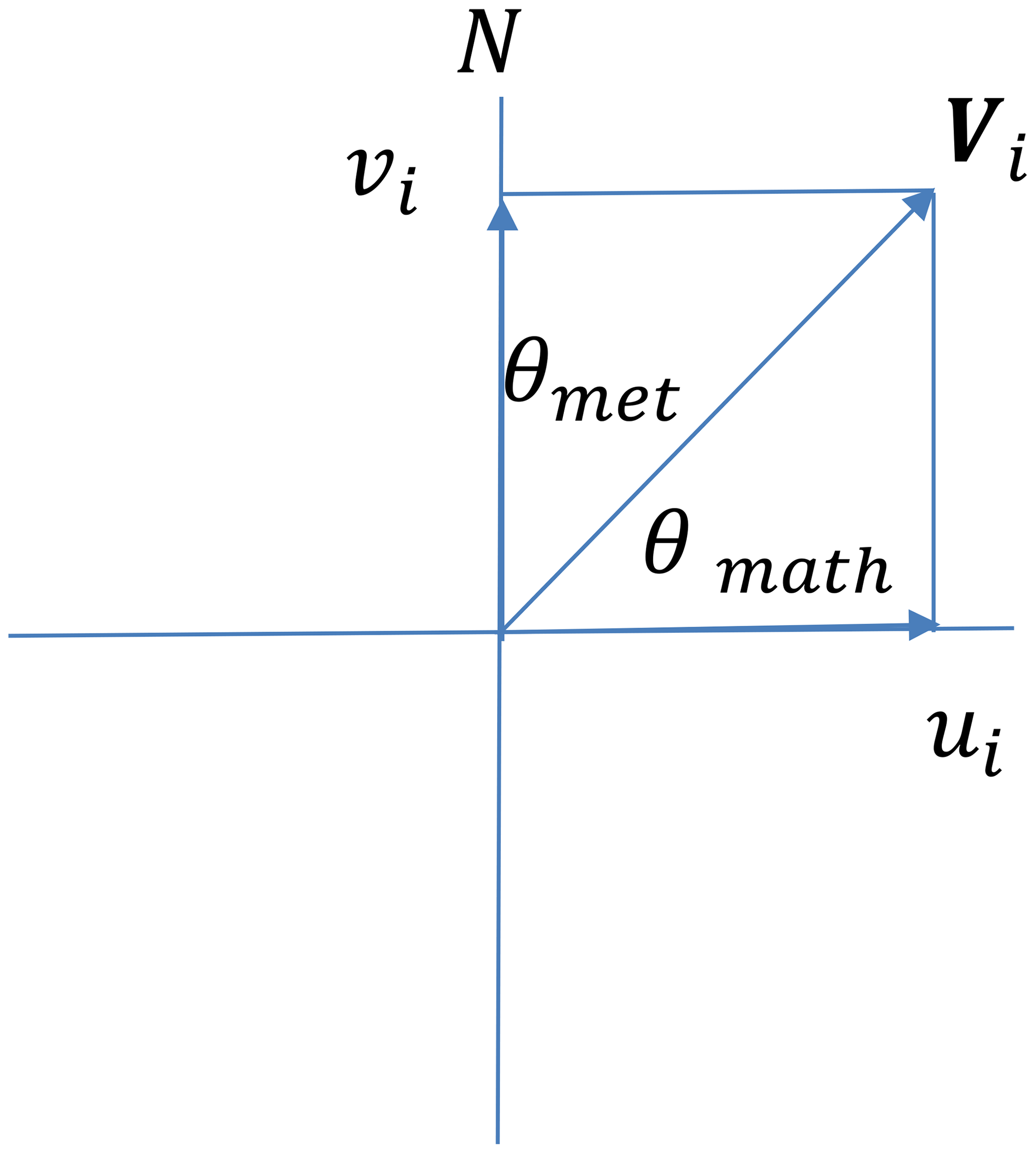
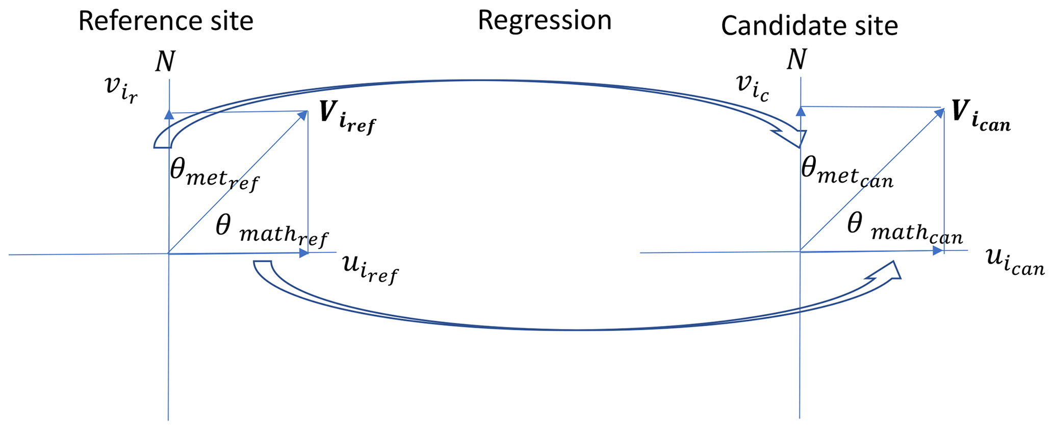
Figure 1 Difference between the meteorological wind direction and the mathematical wind direction and the component of the wind vector.

In some studies, it is necessary for any wake model used to be straightforward, dependent on relatively few wake measurements and economic in terms of the necessary computing power. Despite their relative simplicity, these models tend to give results which are in reasonable agreement with the available data in the case of a single wake within a small wind farm and a simple meteorological environment. In addition, a comparison of different wake models does not suggest any particular difference in terms of accuracy between the sophisticated and simplified models (Manwell et al., 2009).

The use of wake models can also be illustrated by considering a semi-empirical model (Katić et al., 1986) that is often used for wind farm output predictions. This model attempts to characterise the energy content in the flow field whilst ignoring the details of the exact nature of the flow field, which is assumed to consist of an expanding wake with uniform velocity deficit that decreases with distance downstream (Manwell et al., 2009).

Figure 2 Calculating the value of ${\mathit{\theta }}_{{\mathrm{met}}_{i_{\mathrm{p}}}}$ according to the value of ${\mathit{u}}_{i_{\mathrm{p}}}$ and ${\mathit{v}}_{i_{\mathrm{p}}}$.

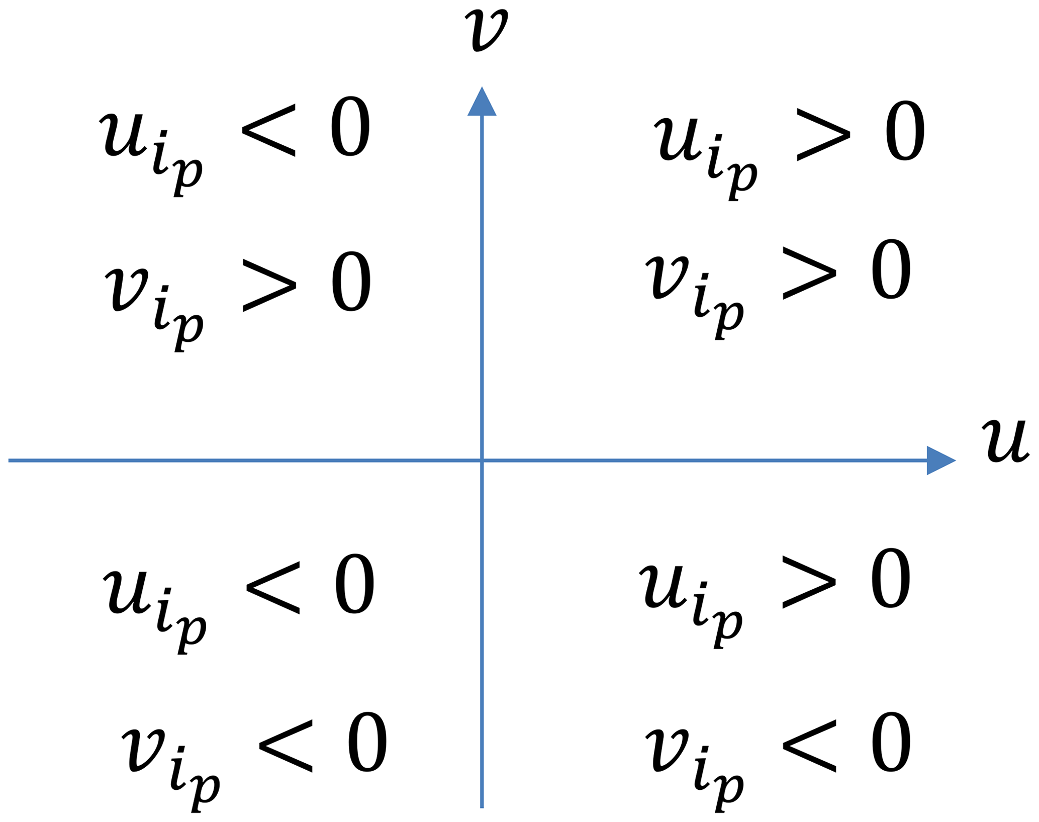
Figure 3 Map of Malta showing relative location of the candidate and the reference sites (Google, 2019) (©Google Maps 2019).

Figure 4 Satellite imagery of the Qalet Marku coastal watch tower, located on a promontory near Bahar ic-Caghaq.

The N.Ø. Jensen wake model (Jensen, 1983) is a simple wake model based on the assumption of a wake with a linear wake cone. The results from this model are comparable to experimental results.

Several metrics may be used to evaluate the accuracy of the models (Rogers et al., 2005a), and it is important to employ more than one metric (Santamaria-Bonfil et al., 2016) to perform the evaluation. The lower the value of the metric, the better the performance of the model. In this case the NMAE and the NMSE were used to quantify the performance of the model. The purpose of using normalised values is to provide results which are independent of wind farm sizes (Madsen et al., 2005).

The NMAE is suitable to describe the errors which are uniformly distributed around the mean, also revealing the average variance between the true value and the predicted value (Hu et al., 2013). The NMAE applies the same weight to the individual errors. The NMSE is a measure of the extent of the dispersion of the errors around the mean and gives a higher weight to larger errors. It assumes that the errors are unbiased and follow a normal distribution (Santamaria-Bonfil et al., 2016). The percentage error of the energy yield gives an estimate of the accuracy of the model for predicting the total energy generated by the wind farm over the period of evaluation. Since each metric has disadvantages that can lead to inaccurate evaluation of the results, it is not recommended to depend only on one measure (Shcherbakov et al., 2013)

Figure 5 View of the wind farm rendered onto an image of the area and also showing the lidar unit.

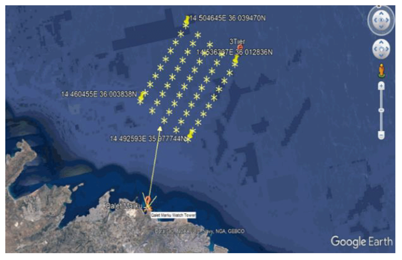
Figure 6 Satellite imagery of the wind farm showing the location of the 50 wind turbines with respect to the coastal lidar station (©Google Maps 2019).

3 Theoretical background

MCP methods are based on regression techniques. Regression can be performed by using MLR. However, as mentioned above, several more powerful techniques exist, amongst which are ANNs, SVR and DTs. While MCP methodologies have been developed for wind speed, they cannot be directly used for predicting wind direction (Bosart and Papin, 2017). Nothing has been found in literature on MCP techniques that explicitly mentions prediction of wind direction at that candidate site. The use of wind speed vectors is a way of using a regression methodology to predict the wind direction, by breaking the wind speed vector into its respective components. MCP methodologies are normally used to predict the wind speed magnitude at the candidate site, but not the direction. Wind velocity may be negative (if one considers it as a vector), and the MCP methodology normally considers the positive value of the wind, i.e. magnitude. The methodology used creates a regression model using the wind velocity vector components to predict the wind vector components at the candidate site (Bosart and Papin, 2017).

Figure 7 Applied methodology.

The methodology is based upon a simple relationship between the meteorological wind direction θ_met and the mathematical wind direction θ_math such that

$$\begin{array}{}\text{(1)}& {\mathit{\theta }}_{\mathrm{math}}=\mathrm{90}-{\mathit{\theta }}_{\mathrm{met}},\end{array}$$

in which the wind speed vector V_i can be broken down into its vector components such that

$$\begin{array}{}\text{(2)}& {\displaystyle }{\mathit{u}}_i=\left|{\mathit{V}}_i\right|\cos {\mathit{\theta }}_{\mathrm{math}}=\left|{\mathit{V}}_i\right|\cos \left(\mathrm{90}-{\mathit{\theta }}_{\mathrm{met}}\right),\text{(3)}& {\displaystyle }{\mathit{v}}_i=\left|{\mathit{V}}_i\right|\sin {\mathit{\theta }}_{\mathrm{math}}=\left|{\mathit{V}}_i\right|\sin \left(\mathrm{90}-{\mathit{\theta }}_{\mathrm{met}}\right),\end{array}$$

in which case the values of u_i and v_i, which may be either positive or negative depending on the direction of the wind (the value of θ_met), are the wind components in the north (y) and the east (x) directions (axes). The relationship is shown in Fig. 1.

Also,

$$\begin{array}{}\text{(4)}& \left|{\mathit{V}}_i\right|={\left({\mathit{u}}_i^{\mathrm{2}}+{\mathit{v}}_i^{\mathrm{2}}\right)}^{\frac{\mathrm{1}}{\mathrm{2}}}.\end{array}$$

The regression is carried out between the respective components of the wind velocity in the y and x directions, hence establishing a relationship between the components at both sites. The forecasted wind direction at the candidate site is then obtained from the forecasted wind components using the relationship in Eq. (5):

$$\begin{array}{}\text{(5)}& {\mathit{\theta }}_{{\mathrm{met}}_{i_{\mathrm{p}}}}=\mathrm{90}-{\tan }^{-\mathrm{1}}{\displaystyle \frac{{\mathit{v}}_{i_{\mathrm{p}}}}{{\mathit{u}}_{i_{\mathrm{p}}}}}.\end{array}$$

The value of the angle ${\mathit{\theta }}_{{\mathrm{met}}_{i_{\mathrm{p}}}}$ depends on the direction of ${\mathit{u}}_{i_{\mathrm{p}}}$ and ${\mathit{v}}_{i_{\mathrm{p}}}$ as shown in Fig. 2 and in accordance with the relationships shown in Eq. (6),

$$\begin{array}{}\text{(6)}& \begin{array}{lll}{\mathit{u}}_{i_{\mathrm{p}}}>\mathrm{0}\mathrm{and}{\mathit{v}}_{i_{\mathrm{p}}}>\mathrm{0}& \mathrm{NE}\mathrm{winds}& \mathrm{0}{}^{\circ }<{\mathit{\theta }}_{{\mathrm{met}}_{i_{\mathrm{p}}}}<\mathrm{90}{}^{\circ }\\ {\mathit{u}}_{i_{\mathrm{p}}}>\mathrm{0}and{\mathit{v}}_{i_{\mathrm{p}}}<\mathrm{0}& \mathrm{SE}\mathrm{winds}& \mathrm{90}{}^{\circ }<{\mathit{\theta }}_{{\mathrm{met}}_{i_{\mathrm{p}}}}<\mathrm{180}{}^{\circ }\\ {\mathit{u}}_{i_{\mathrm{p}}}<\mathrm{0}\mathrm{and}{\mathit{v}}_{i_{\mathrm{p}}}<\mathrm{0}& \mathrm{SW}\mathrm{winds}& \mathrm{180}{}^{\circ }<{\mathit{\theta }}_{{\mathrm{met}}_{i_{\mathrm{p}}}}<\mathrm{270}{}^{\circ }\\ {\mathit{u}}_{i_{\mathrm{p}}}<\mathrm{0}\mathrm{and}{\mathit{v}}_{i_{\mathrm{p}}}>\mathrm{0}& \mathrm{NW}\mathrm{winds}& \mathrm{270}{}^{\circ }<{\mathit{\theta }}_{{\mathrm{met}}_{i_{\mathrm{p}}}}<\mathrm{360}{}^{\circ },\end{array}\end{array}$$

and Eq. (7),

$$\begin{array}{}\text{(7)}& \begin{array}{lll}{\mathit{u}}_{i_{\mathrm{p}}}=\mathrm{0}\mathrm{and}{\mathit{v}}_{i_{\mathrm{p}}}>\mathrm{0}& \left(\mathrm{North}\mathrm{wind}\right)& {\mathit{\theta }}_{{\mathrm{met}}_{i_{\mathrm{p}}}}=\mathrm{0}{}^{\circ }\\ {\mathit{u}}_{i_{\mathrm{p}}}=\mathrm{0}\mathrm{and}{\mathit{v}}_{i_{\mathrm{p}}}<\mathrm{0}& \left(\mathrm{South}\mathrm{wind}\right)& {\mathit{\theta }}_{{\mathrm{met}}_{i_{\mathrm{p}}}}=\mathrm{180}{}^{\circ }\\ {\mathit{u}}_{i_{\mathrm{p}}}>\mathrm{0}\mathrm{and}{\mathit{v}}_{i_{\mathrm{p}}}=\mathrm{0}& \left(\mathrm{East}\mathrm{wind}\right)& {\mathit{\theta }}_{{\mathrm{met}}_{i_{\mathrm{p}}}}=\mathrm{90}{}^{\circ }\\ {\mathit{u}}_{i_p}<\mathrm{0}\mathrm{and}{\mathit{v}}_{i_{\mathrm{p}}}=\mathrm{0}& \left(\mathrm{West}\mathrm{wind}\right)& {\mathit{\theta }}_{{\mathrm{met}}_{i_{\mathrm{p}}}}=\mathrm{270}{}^{\circ }.\end{array}\end{array}$$

The results are compared by using the NMAE and the NMSE of the residuals, using Eqs. (8) to (12). The residuals e_i are the errors between the predicted and the actual output power values from the wind farm,

$$\begin{array}{}\text{(8)}& e_i=P_i-P_{{\mathrm{act}}_i}.\end{array}$$

The formula used to calculate the NMAE is shown in Eq. (9), whereby the errors are normalised by dividing by the average power production over the whole period of evaluation (Madsen et al., 2005):

$$\begin{array}{}\text{(9)}& \mathrm{NMAE}={\displaystyle \frac{{\sum }_{i=\mathrm{1}}^N\left|e_i\right|}{{\sum }_{i=\mathrm{1}}^N{P}_i}}.\end{array}$$

The NMSE is given by

$$\begin{array}{}\text{(10)}& \mathrm{NMSE}={\displaystyle \frac{\frac{\mathrm{1}}{N}{\sum }_{i=\mathrm{1}}^N{\left(e_i\right)}^{\mathrm{2}}}{\stackrel{\mathrm{‾}}{P}\cdot \stackrel{\mathrm{‾}}{P_{\mathrm{act}}}}},\end{array}$$

where

$$\begin{array}{}\text{(11)}& \stackrel{\mathrm{‾}}{P}={\displaystyle \frac{\mathrm{1}}{N}}{\sum }_{i=\mathrm{1}}^N{P}_i\end{array}$$

and

$$\begin{array}{}\text{(12)}& \stackrel{\mathrm{‾}}{P_{\mathrm{act}}}={\displaystyle \frac{\mathrm{1}}{N}}{\sum }_{i=\mathrm{1}}^N{P}_{{\mathrm{act}}_i}.\end{array}$$

The percentage error in overall energy yield is given by Eq. (13), where

$$\begin{array}{}\text{(13)}& e_{\mathrm{eng}}=\left({\displaystyle \frac{{\sum }_{i=\mathrm{1}}^N{P}_i-{\sum }_{i=\mathrm{1}}^N{P}_{{\mathrm{act}}_i}}{{\sum }_{i=\mathrm{1}}^N{P}_{{\mathrm{act}}_i}}}\right)\cdot \mathrm{100}\mathit{\%}.\end{array}$$

Figure 8 Application of regression methodologies to wind direction.

Figure 9 Predicting the wind direction.

4 A case study – site conditions and the modelled offshore wind farm

4.1 The reference and candidate sites

The reference site employed in this study is the Meteorological Office at Malta International Airport (MIA), Luqa, and the candidate site is comprised of data collected by a ZephIR 300 lidar (https://www.zxlidars.com/wind-lidars/zx-300/, last access: 10 May 2020) unit administered by the University of Malta's Institute for Sustainable Energy. The unit was situated on the roof of a coastal watch tower at Qalet Marku, situated in the northern part of the island of Malta (Mifsud et al., 2018). The relative location of the two sites is shown in Fig. 3, while Fig. 4 shows a satellite image of the location of the coastal watch tower.

Tables 1 and 2 show the properties of the candidate and the reference sites respectively (Cordina et al., 2017; Mifsud et al., 2018). In this case the wind data measured by the lidar at a height of 80 m would be equivalent to a cumulative height of 100 m above sea level, which would be the hub height of the wind turbines in the wind farm. This is because the lidar is situated on the rooftop of a coastal tower at a height of 20 m above sea level, as shown in Table 3.

Table 1 Candidate site parameters (Cordina et al., 2017).

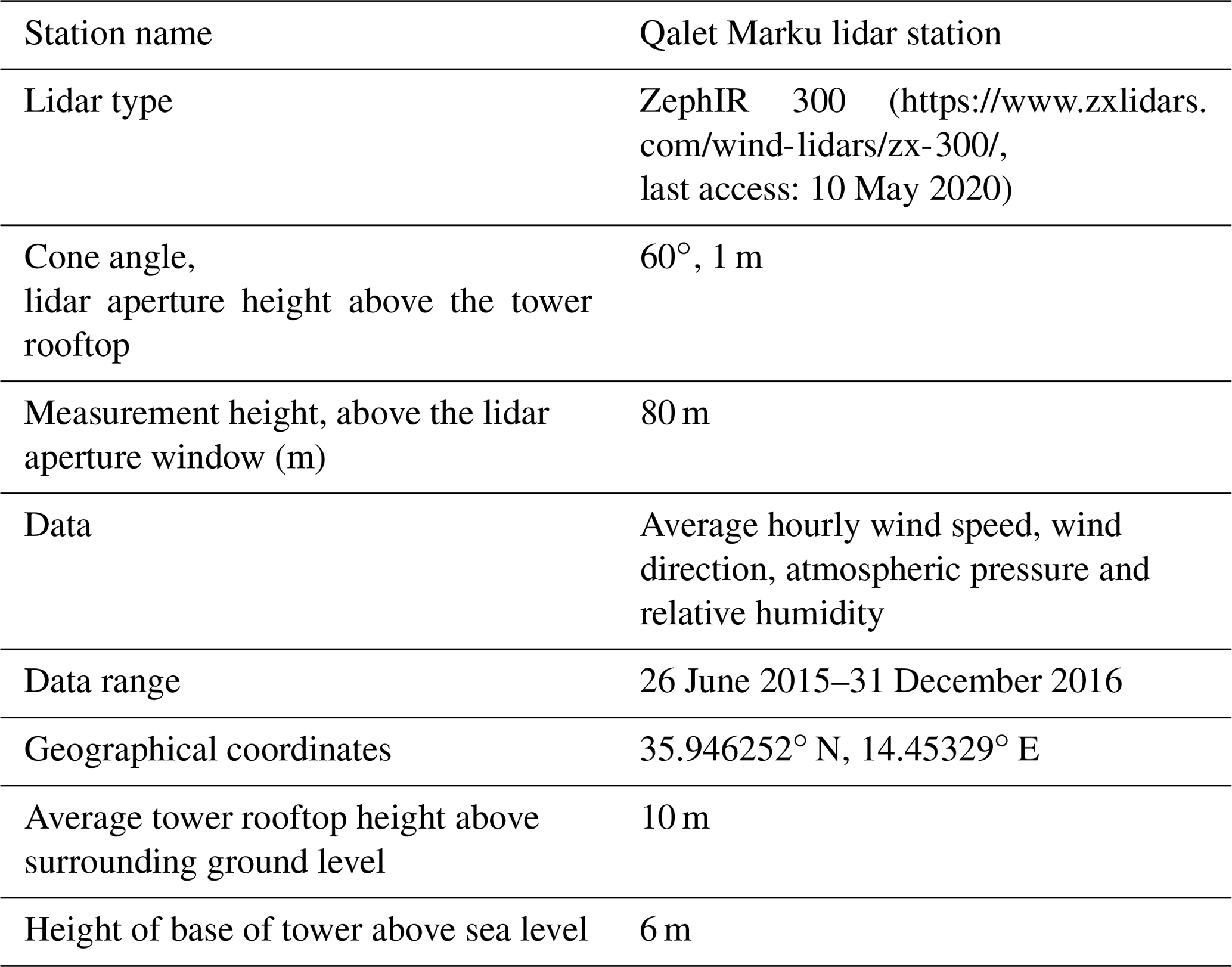
Table 2 Reference site parameters (Malta International Airport).

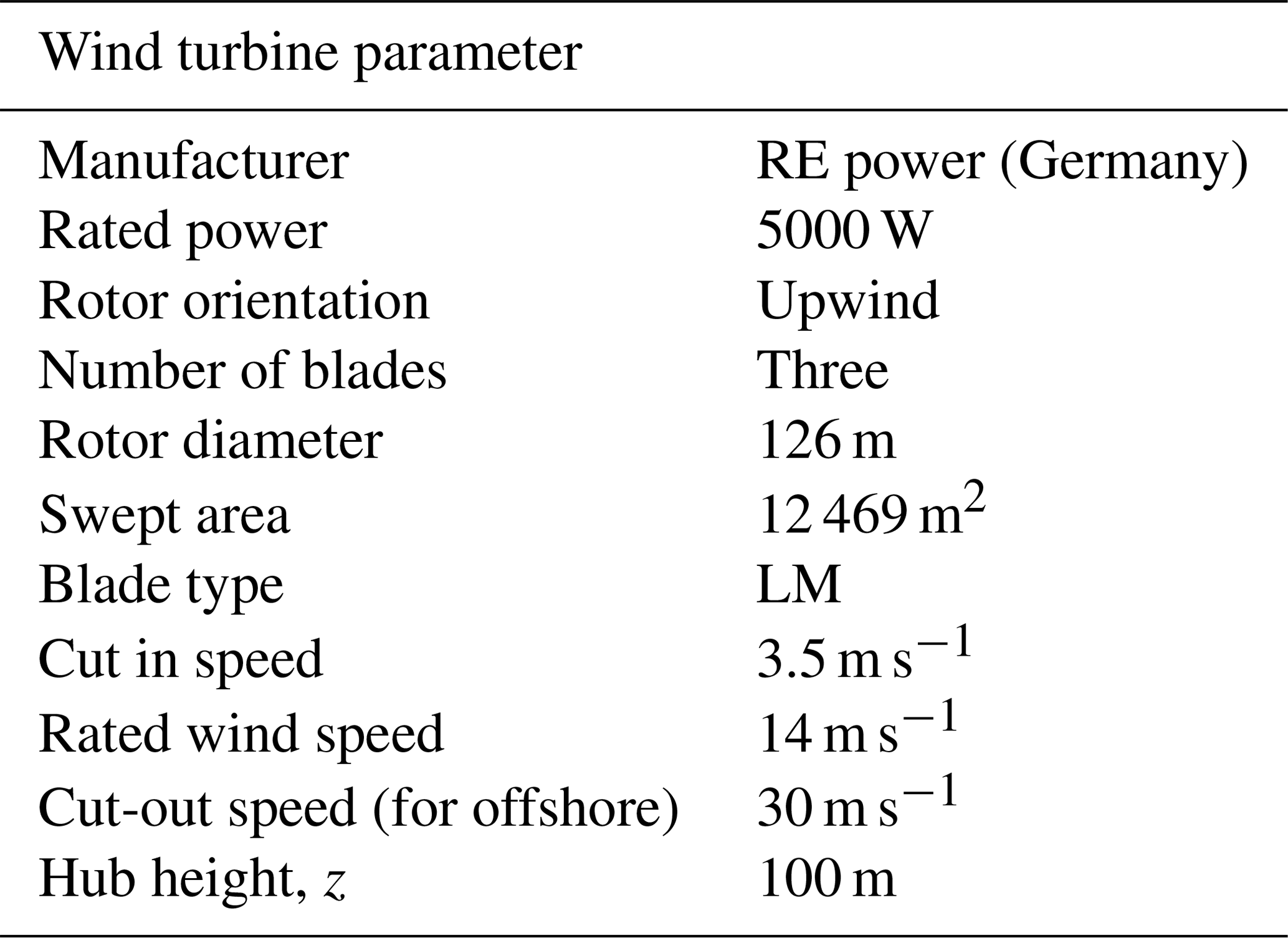
Table 3 Wind turbine parameters used in the study (https://wind-turbine-models.com, last access: 10 May 2020).

4.2 The available wind data

The measurement campaign at the candidate site started on 1 July 2015 and ended on 31 December 2016. Hourly wind data were available for this time period from both the reference and candidate sites. The ideal number of data points used to create the MCP models is thus 8784, i.e. the number of hours in 2016. Following analysis and filtration of the wind speed data at the reference site, 98 % of the data were considered suitable for the creation of the model. The data at the reference site were all considered suitable. Hence, the regression model was created using the concurrent 8616 wind speed and direction values. For the year 2015, 95.6 % of the data were considered valid (the measurement campaign started on 26 June 2015; hence there were 4368 h of wind speed and direction measurements of which 4176 were valid data points).

The MCP analysis was carried out using both wind speed and wind direction. The data from the reference site were used as the independent data set. The models were created using the data for the year 2016, while the reference site wind data for 2015 were used to create the predicted wind speed and wind direction as inputs to the wind farm model.

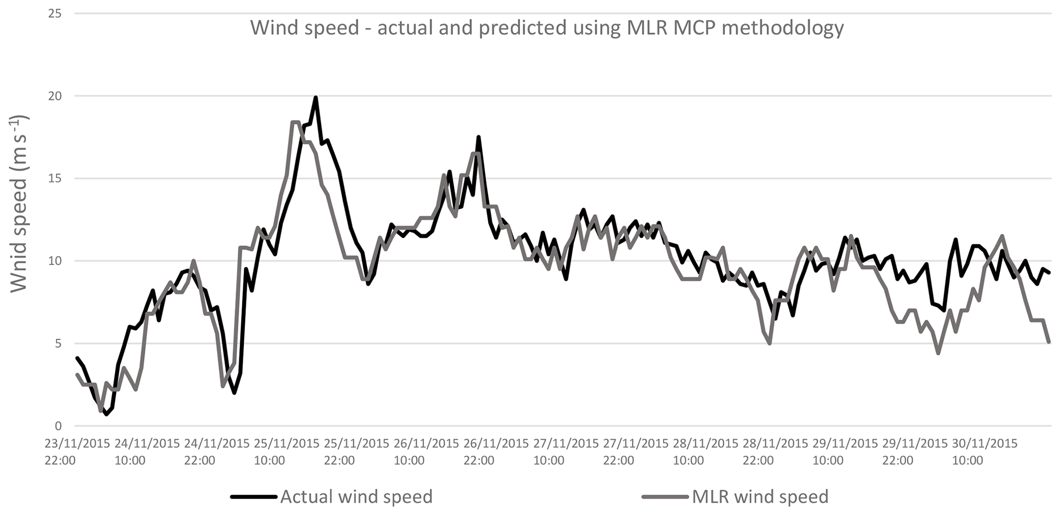
Figure 10 Comparing actual wind speed and wind speed predicted by MLR methodology with wind data for 2015.

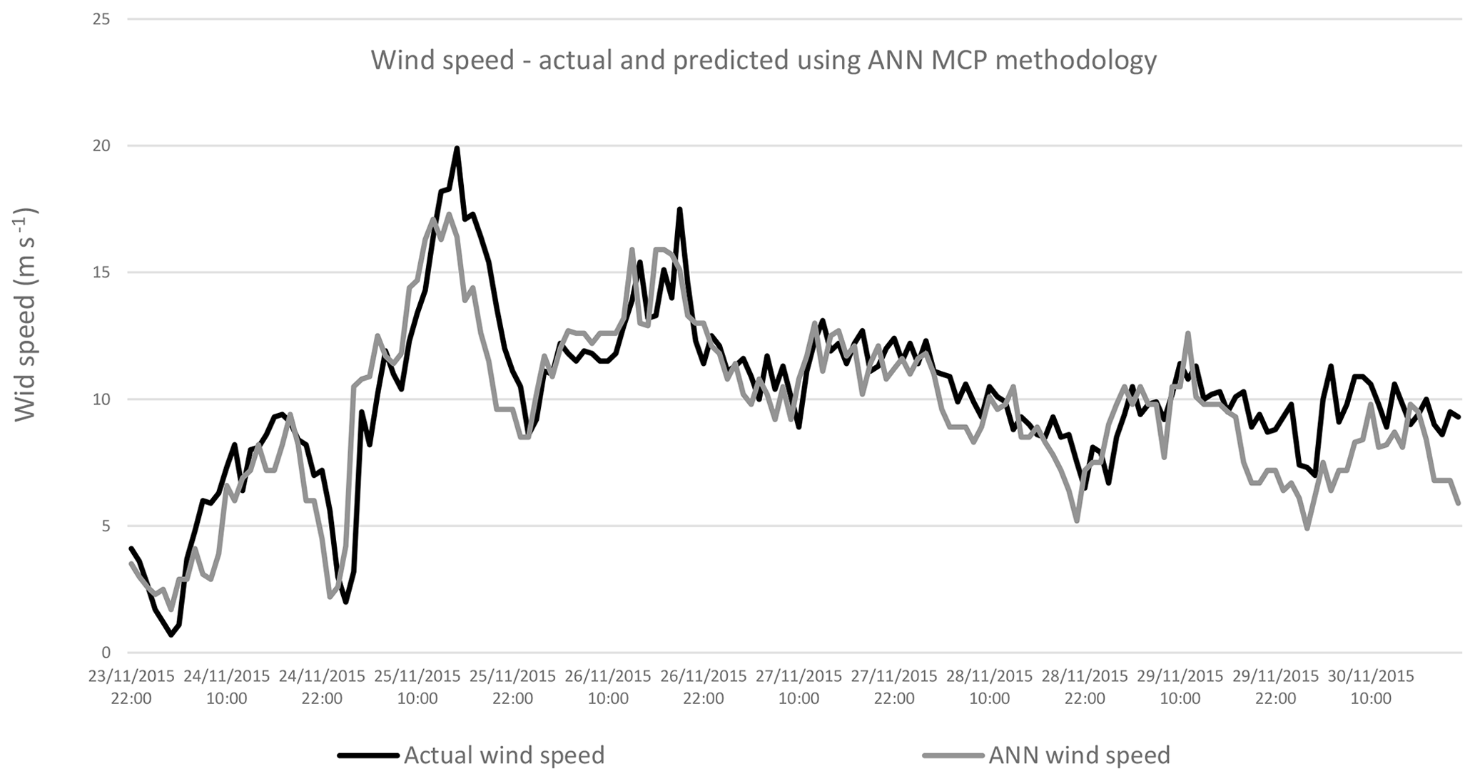
Figure 11 Comparing actual wind speed and wind speed predicted by ANN methodology with wind data for 2015.

4.3 The wind farm design in windPRO^®

The hypothetical wind farm is located opposite the coastal watch tower of Qalet Marku (35.945892^∘ N, 14.452498^∘ E). WindPRO^® 2.7 was used to render an image of the wind farm onto an image of the lidar unit taken from the watch tower. This gives an indication as to the extent of the wind farm. This is shown in Fig. 5 while Fig. 6 shows the satellite imagery of the wind farm, showing a 250 MW capacity wind farm. The wind farm faces the northwest direction, which is the prevailing wind direction.

The wind farm is made up of 50 wind turbines. There are 10 wind turbines in a row, having a cross-wind spacing of five rotor diameters (5D). The distance between the successive rows of wind turbines, or the downwind spacing, is eight rotor diameters (8D). Thus, considering wind turbines with a rotor diameter, D, of 126 m (for a 5 MW wind turbine), the distance between the turbines in the cross-wind direction is 630 m, and the distance between successive rows of wind turbines in the downwind direction is 1008 m. The wind turbine selected for use in windPRO^® is the REpower 5 MW wind turbine whose parameters are shown in Table 3.

Table 4 Description of the regression methodologies used for the measure–correlate–predict methodology.

5 Methodology

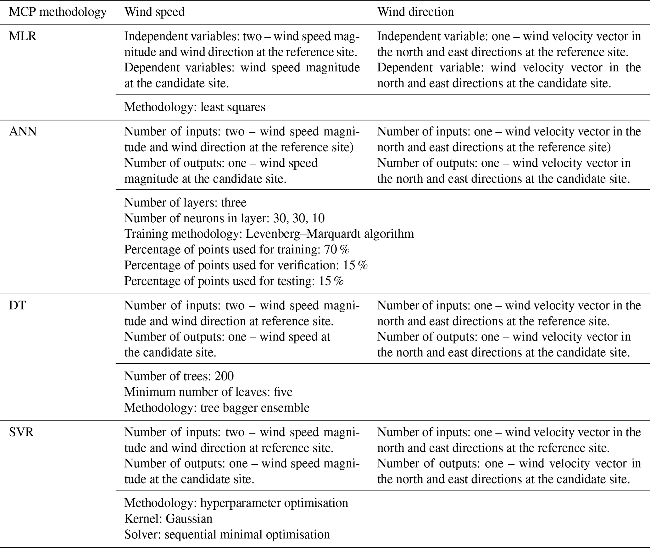
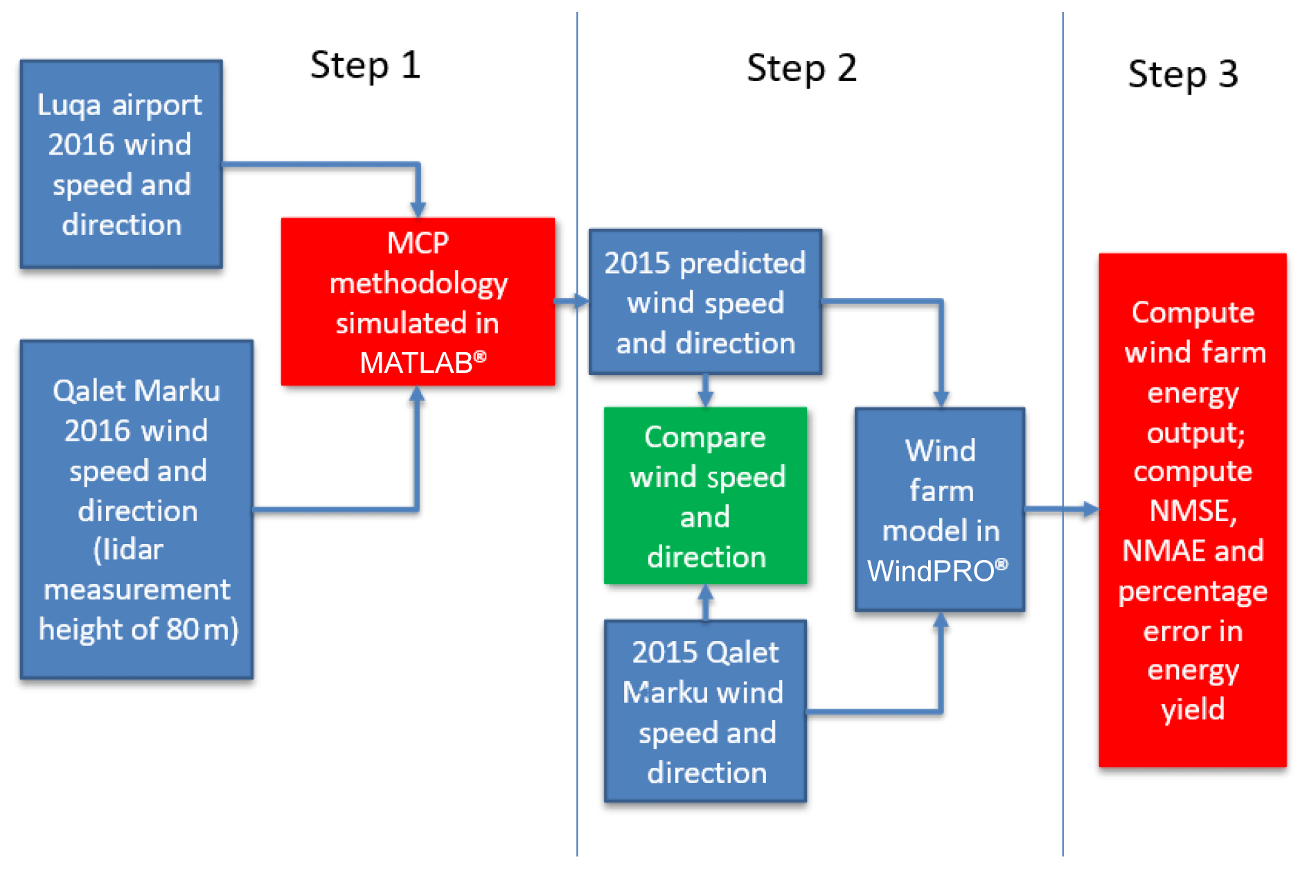
Figure 7 shows the methodology applied in this paper. The study is divided into three steps as follows.

1. Step 1. The various MCP methodologies are used to compute the MCP model. For wind speed, the models are trained using wind speed and direction data at candidate and reference sites for the year 2016. For the wind direction the input training data are the wind velocity vector component in the north or east direction at the candidate site, and the output of the model is the respective component at the candidate site. The models are summarised in Table 4. Table 4 describes the inputs used to train the respective models, for both wind speed and wind direction. It also shows the parameters of the models and the algorithms used to train the model, such as least squares for MLR and the Levenberg–Marquardt algorithm for ANNs.

2. Step 2. The 2015 wind speed and wind direction are predicted using the models computed in Step 1. The predicted and actual wind speed and wind direction are used to compute the power output from the wind farm. This is done by feeding the wind speed and direction data into the windPRO^® model.

3. Step 3. Compute and compare the normalised mean-squared error (NMSE), normalised absolute error (NMAE) and percentage error in the power.

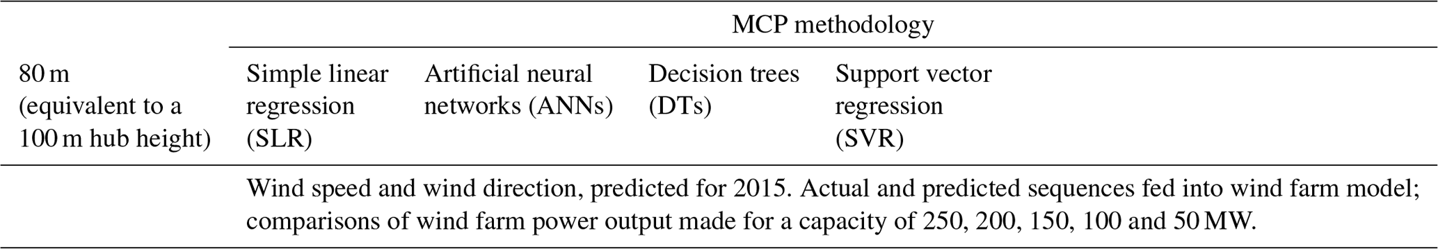
The combinations of lidar measurement heights and MCP methodologies are shown in Table 5.

Regression models were created for the MCP methodologies using the reference and candidate wind speed and direction for the year 2016. These regression models were created using MLR, ANNs, DTs and SVR. A model was created for both wind speed and direction.

Table 5 Summary of combinations of methodologies, lidar measurement heights and amount of wind turbines used in the analysis.

The wind speed and wind direction for 2015 were then predicted with the models by feeding the speed and direction values from the reference site from the year 2015. Thus, a sequence of predicted wind speeds and wind direction time series could be compared to the actual speed and direction measured at the candidate site for the year 2015. The models for the wind speed and the wind direction are independent of each other.

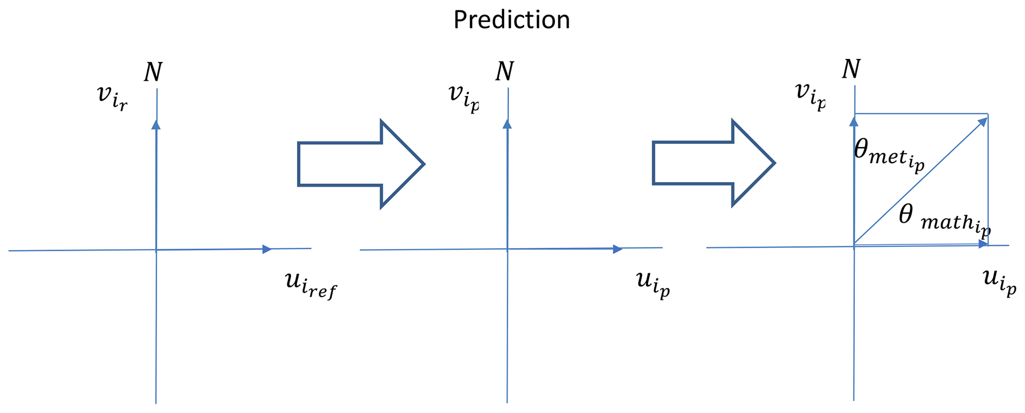
In the case of wind direction, the MCP methodologies are applied as shown in Figs. 8 and 9. Figure 8 shows that two regressions are carried out: one for the magnitude of the wind component in the north direction and one for the wind component in the east direction. Thus, two models are created using the wind speed and direction data of the reference and the candidate sites for 2016. The two models are then used to derive the predicted wind direction for 2015 at the candidate site as shown in Fig. 9, by using the wind components at the reference site for 2015 as inputs to the respective models. The values of the wind speed in the north direction and the east direction are first predicted, and the wind direction at the candidate site for 2015, ${\mathit{\theta }}_{{\mathrm{met}}_{\mathrm{p}}}$, is then derived from the mathematical relationships given in Eqs. (6) and (7).

Table 6 Summarised results for normalised mean absolute error (NMAE) by MCP methodology and wind farm capacity.

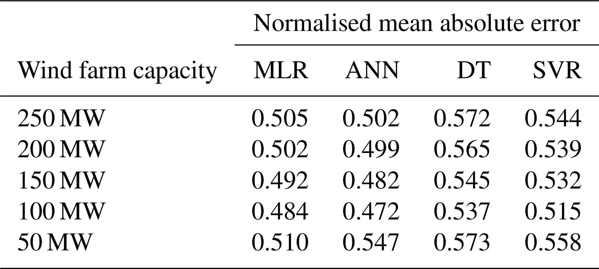
Table 7 Summarised results for the normalised mean-squared error (NMSE) by MCP methodology and wind farm capacity.

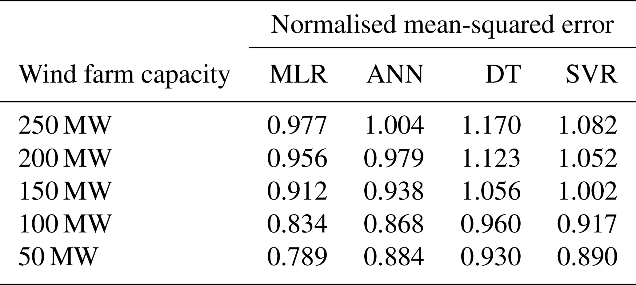
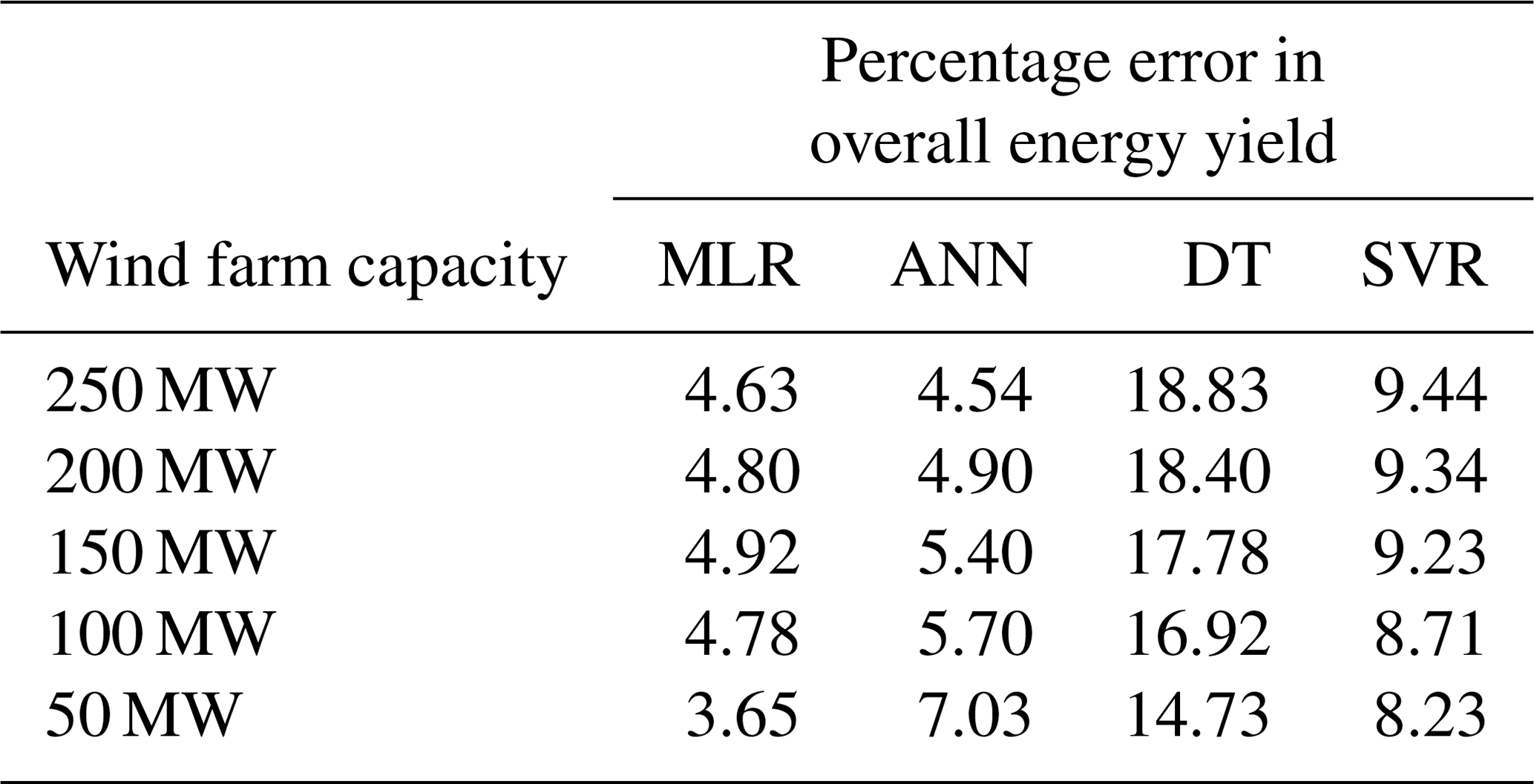
Table 8 Summarised results for percentage error in overall energy yield by MCP methodology and wind farm capacity.

The sequences of wind speed and wind directions (both actual and predicted) were fed into the wind farm model. This was done for different combinations of methodology and wind farm (250, 200, 150, 100 and 50 MW) configurations. The results were compared to determine which combination of MCP methodology and wind farm capacity would give the lowest prediction error. The prediction error for the power output from the wind farm is analysed using the normalised mean-squared error (MSE), the normalised mean absolute error (NMAE) and the percentage error in the overall energy yield for the period of analysis. The results are shown in the following section.

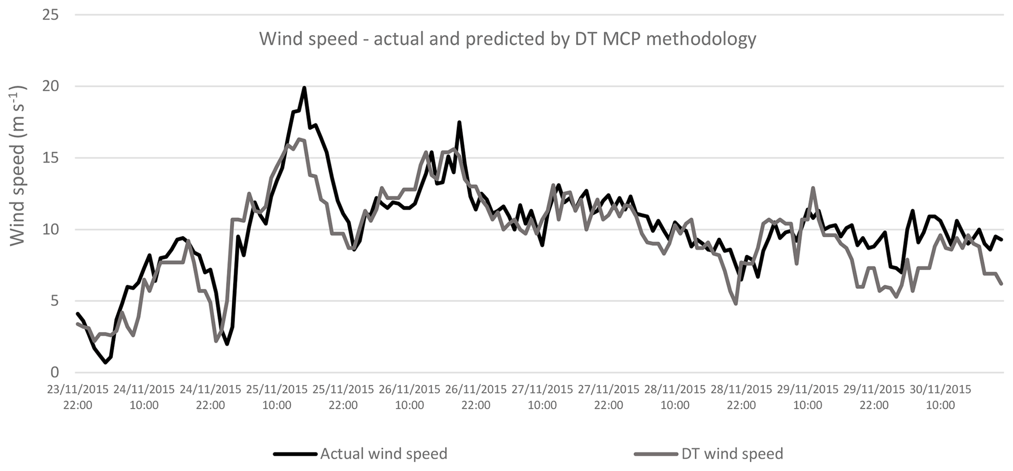
Figure 12 Comparing actual wind speed and wind speed predicted by ANN methodology with wind data for 2015.

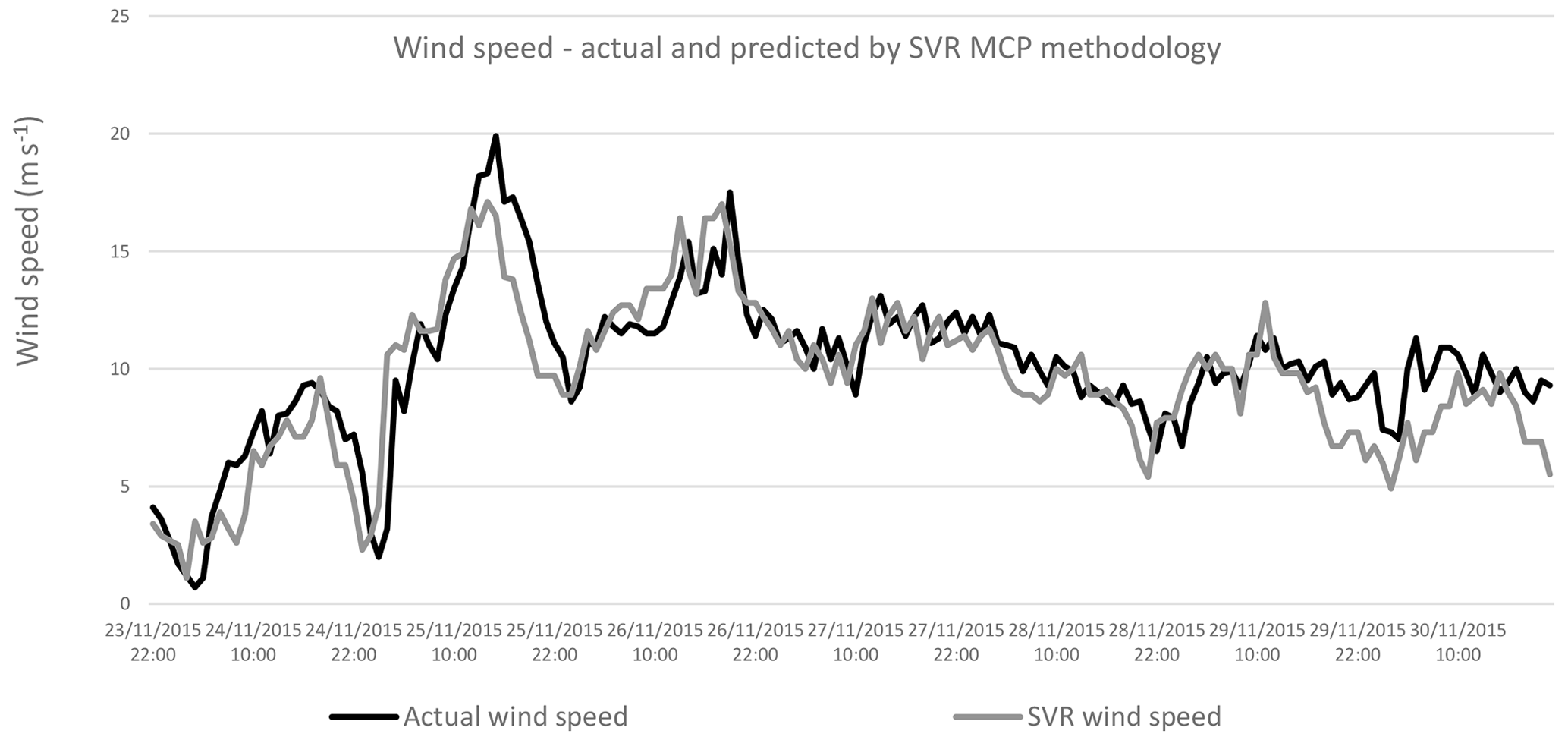
Figure 13 Comparing actual wind speed and wind speed predicted by SVR methodology with wind data for 2015.

Figure 14 Comparing actual and predicted wind direction predicted by MLR methodology with wind data for 2015.

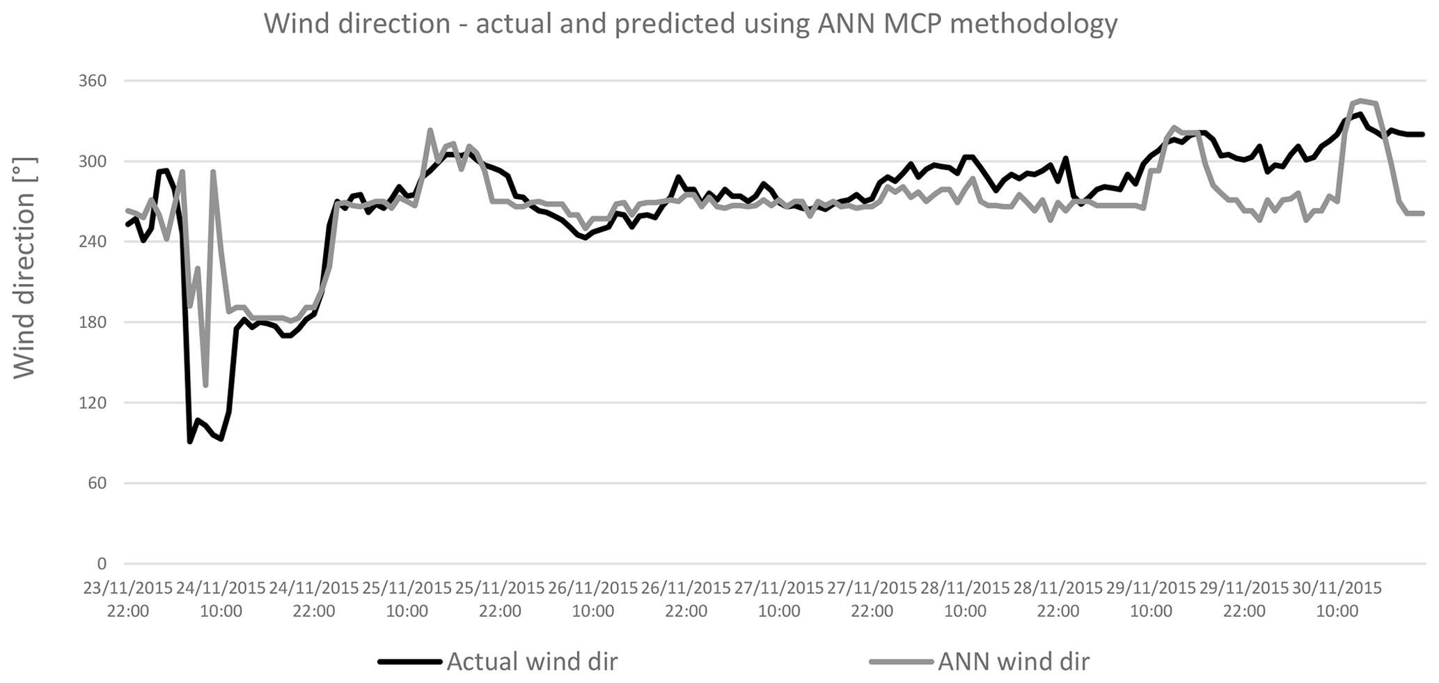
Figure 15 Comparing actual and predicted wind direction predicted by ANN methodology with wind data for 2015.

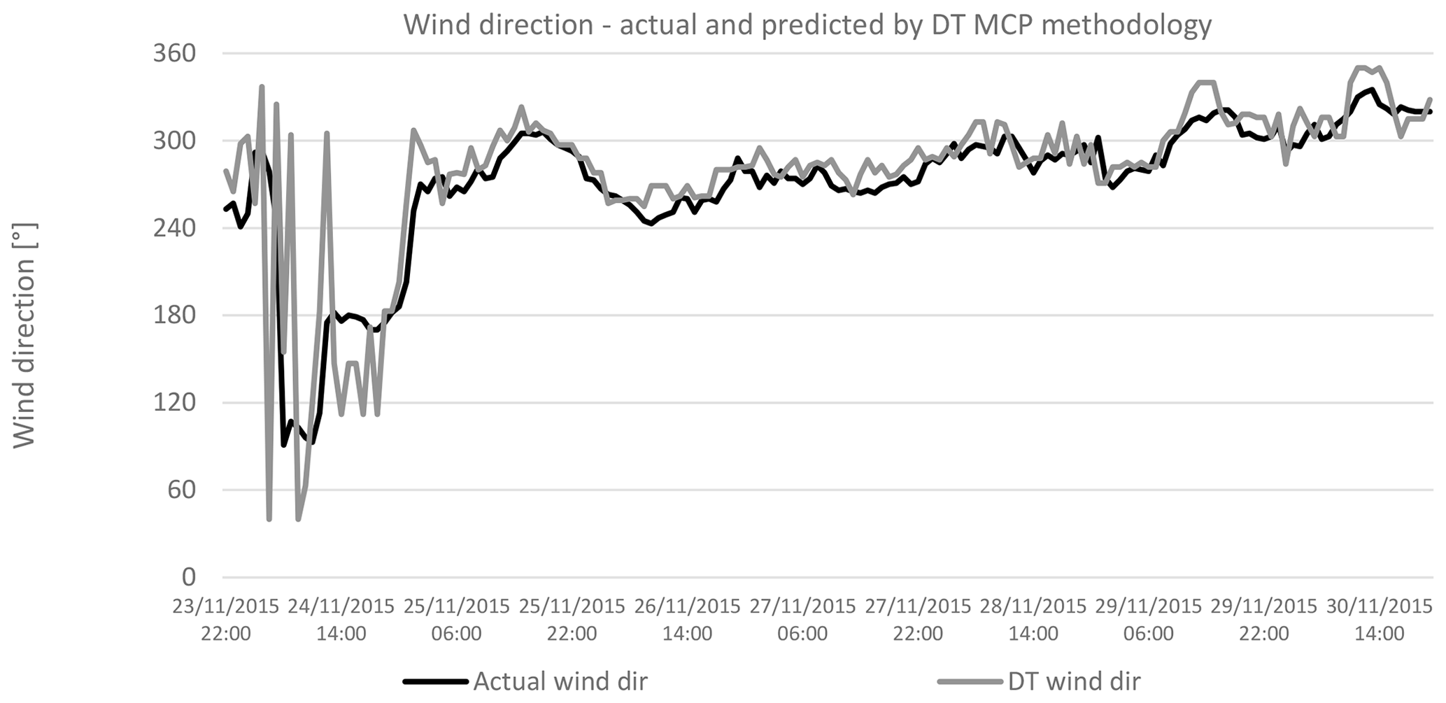
Figure 16 Comparing actual and predicted wind direction predicted by DT methodology with wind data for 2015.

6 Results

A summary of the results is shown below where sequences of data for a specific period of 2015 are compared. These sequences are for wind speed, wind direction and power output. All NMSE, NMAE and percentage errors in the overall energy yield are then shown in the following tables.

6.1 Wind speed and wind direction with MCP methodology

6.1.1 Wind speed with MCP methodology

Figures 10 to 13 show the wind speed from the period 23–30 November 2015. The particular period is chosen because of the high availability of wind. The actual wind data are compared with those predicted by the MLR, ANN, DT and SVR methodologies. The predicted wind values closely follow the actual wind values, for all the MCP methodologies applied.

6.1.2 Wind direction with MCP methodology

Figures 14 to 17 show the wind direction from the period 23–30 November 2015. As above, the actual wind direction at the candidate site is compared to that predicted by the MLR, ANN, DT and SVR methodologies. Again, as in the case for wind speed, there is a similarity between the actual and predicted wind direction values, in all cases.

6.2 Wind farm power output with MCP methodology, for a wind farm capacity of 250 MW

Figures 18 to 21 compare the output power from the wind farm, which is derived from the actual wind speed and wind direction, to the power output derived from the predicted wind speed and direction. This comparison is carried out for the MLR, ANN, DT and SVR methodologies. The results for a wind farm capacity of 250 MW are being shown. As in the case for wind speed and direction, the predicted power output closely follows that obtained with the actual wind speed and direction.

A wind data analysis, carried out using windPRO^®, is shown in the next section. The results presented are a Weibull distribution for wind speed and the wind rose. These charts are computed from the wind speed and direction which are predicted by using the MLR, ANN, DT and SVR MCP methodologies. Thus, the predicted wind speed and direction are compared with the results computed from the actual wind data.

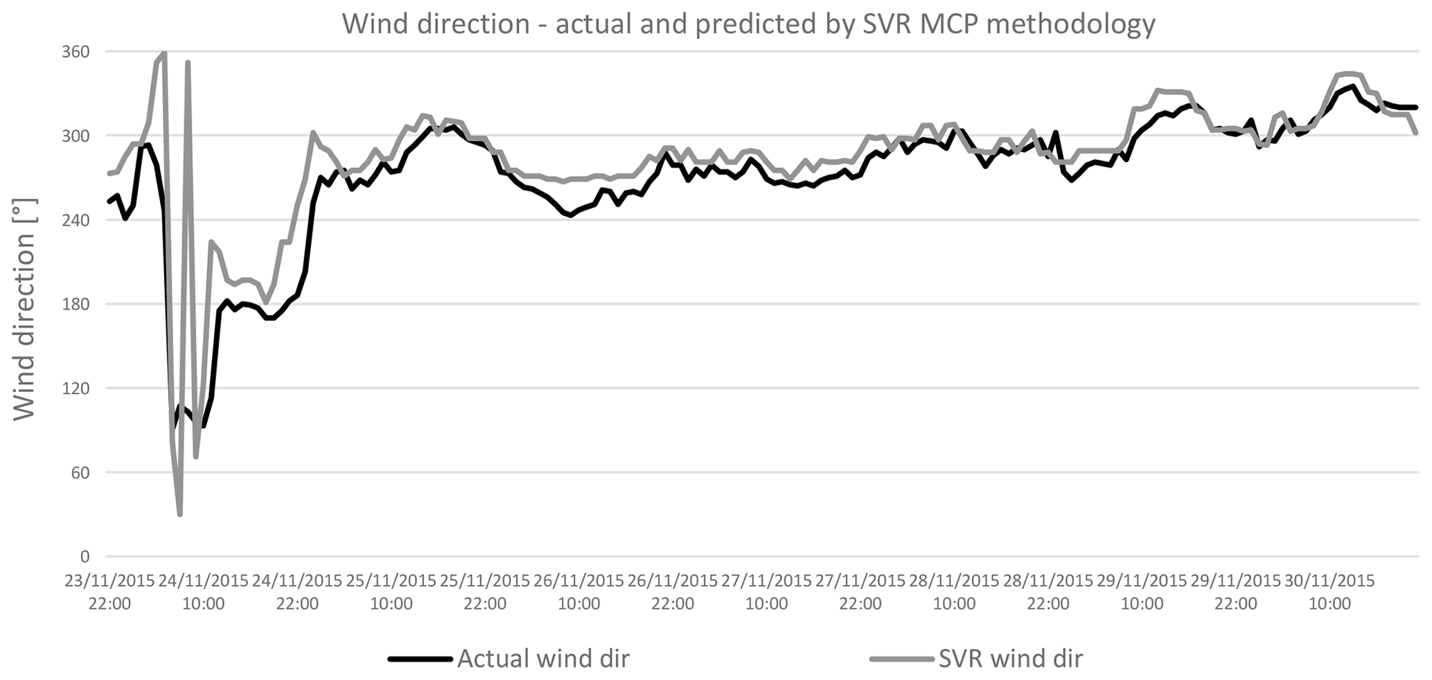
Figure 17 Comparing actual and predicted wind direction predicted by SVR methodology with wind data for 2015.

Figure 18 Comparing actual and predicted power output from the wind farm with wind data for 2015, actual and predicted by MLR methodology.

6.3 The actual wind data for 2015 measured by the lidar system

Figure 22 shows the wind data analysis report from windPRO^® for the actual lidar data measured at the 80 m level height (equivalent to a hub height of 100 m). The images show the Weibull distribution for the wind speed and the wind rose. The reports are used to compare the properties of the actual wind measurements and the predicted wind speed and direction.

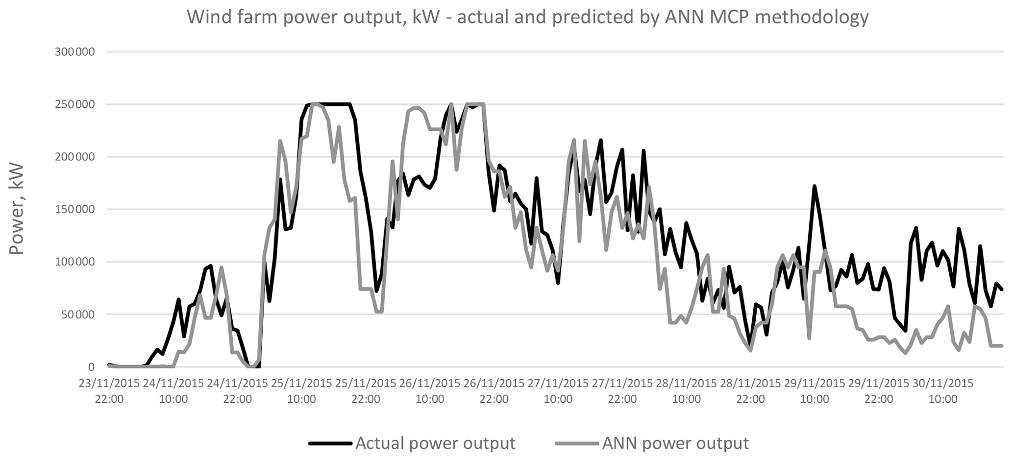
Figure 19 Comparing actual and predicted power output from the wind farm with wind data for 2015, actual and predicted by ANN methodology.

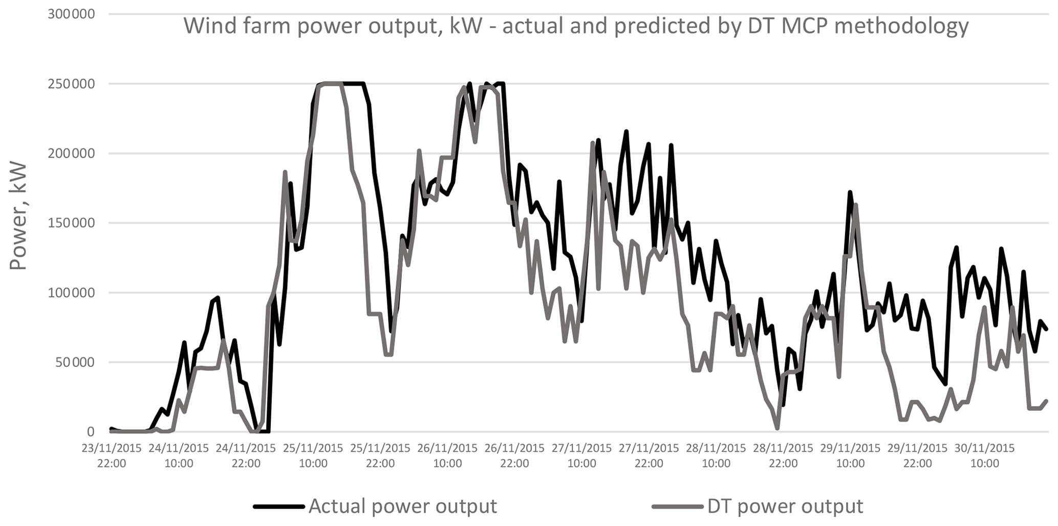
Figure 20 Comparing actual and predicted power output from the wind farm with wind data for 2015, actual and predicted by DT methodology.

A wind data analysis, carried out using windPRO^®, is shown in the next section. The results presented are a Weibull distribution for wind speed and the wind rose. These charts are computed from the wind speed and direction which are predicted by using the MLR, ANN, DT and SVR MCP methodologies. Thus, the predicted wind speed and direction are compared with the results computed from the actual wind data.

6.4 Wind speed and direction predicted using the MCP methodologies

Figures 23 to 26 represent the Weibull distribution and the wind rose for the wind speed and direction predicted by the MLR, ANN, DT and SVR MCP methodologies respectively at the hub height of 100 m. There is a similarity between the Weibull plots for the actual wind data and those for the predicted wind speed, for the same measurement period. Meanwhile, the wind direction predicted by the ANN and DT methodologies shows a higher resemblance to that of the actual wind direction than that predicted by the MLR or SVR methodologies. Hence it is expected that the ANN and the DT methodologies would yield the least error in the predicted power output from the wind farm.

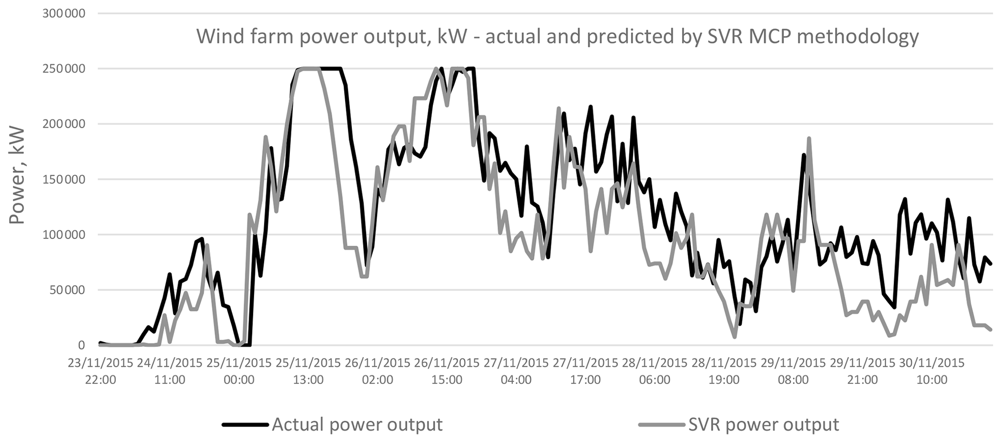
Figure 21 Comparing actual and predicted power output from the wind farm with wind data for 2015, actual and predicted by SVR methodology.

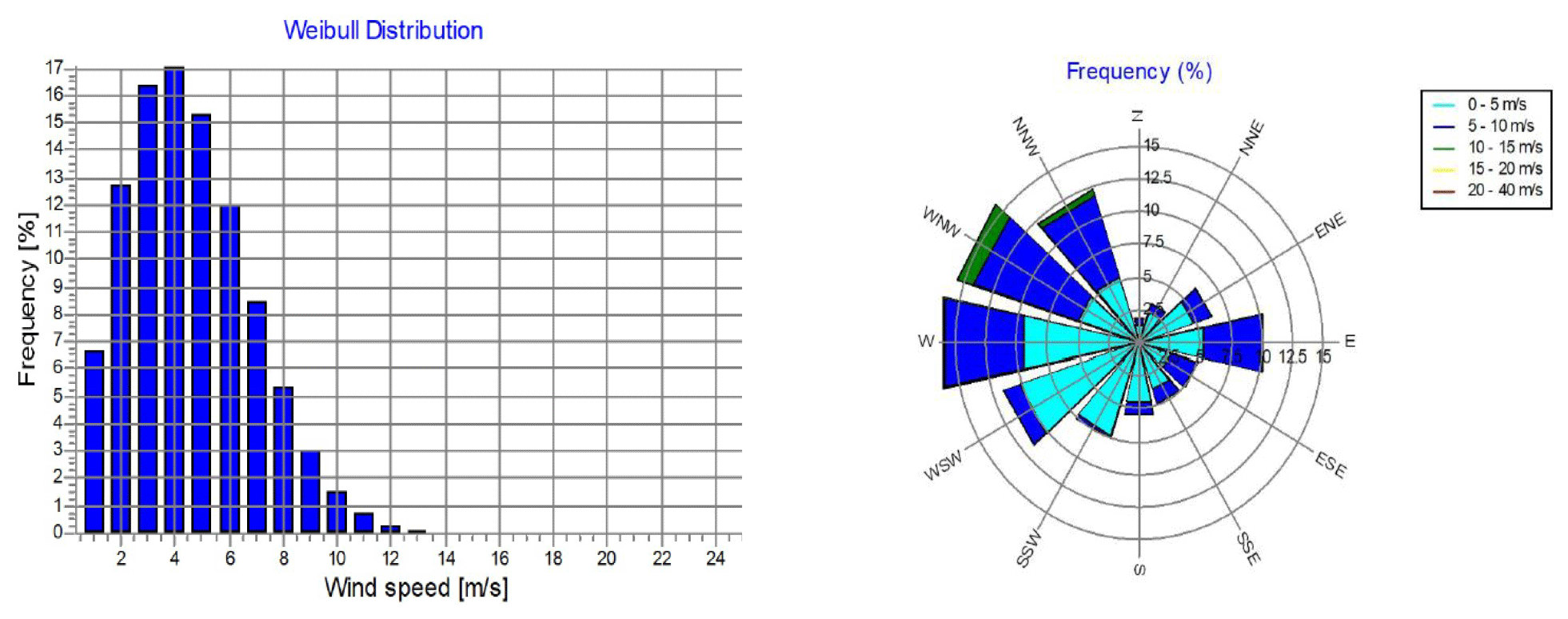
Figure 22 The windPRO^® wind data analysis using actual wind data measured by the lidar equipment at a height of 100 m.

Figure 23 The windPRO^® wind data analysis using wind data predicted by MCP applying MLR at a hub height of 100 m.

The results for the NMAE, the NMSE and the percentage error in the overall energy yield are summarised in Tables 6 to 8. The tables show that the MLR and ANN methodologies have the best performance in NMAE, NMSE and percentage error for energy yield. The results are consistent for all wind farm capacities under consideration. ANNs are better than MLR in the case of NMAE, while MLR is slightly better than ANNs in the case of the 50 MW wind farm capacity. MLR is superior to ANNs in the case of NMSE for all wind farm capacities. However, the differences between the MLR and the ANN methodologies are minimal, and both methodologies show a better performance than the DT or SVR methodologies, especially in the case of the overall energy yield as shown in Table 8. Graphical results are also shown in Figs. 27 to 29.

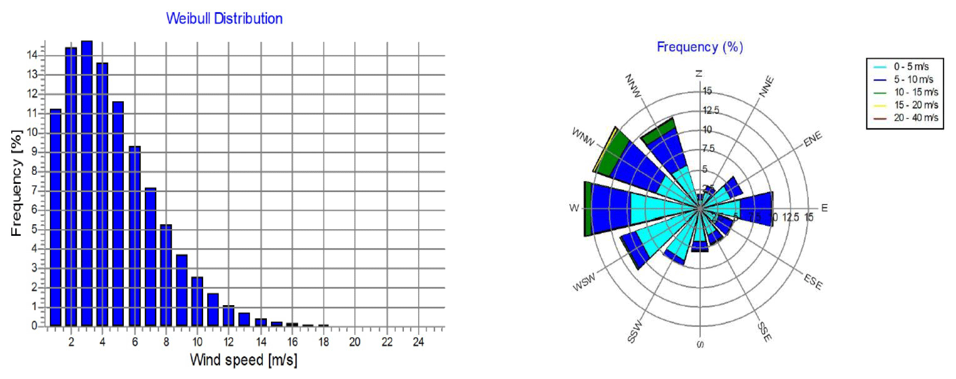
Figure 24 The windPRO^® wind data analysis using wind data predicted by MCP applying ANNs at a hub height of 100 m.

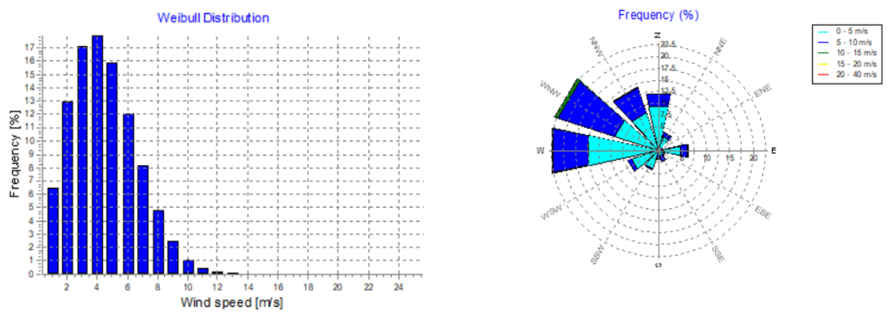
Figure 25 The windPRO^® wind data analysis using wind data predicted by MCP applying DTs at a hub height of 100 m.

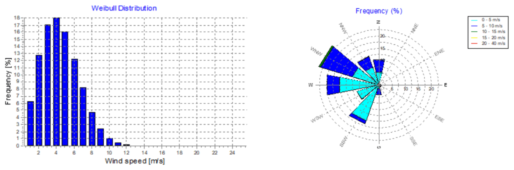
Figure 26 The windPRO^® wind data analysis using wind data predicted by MCP applying SVR at a hub height of 100 m.

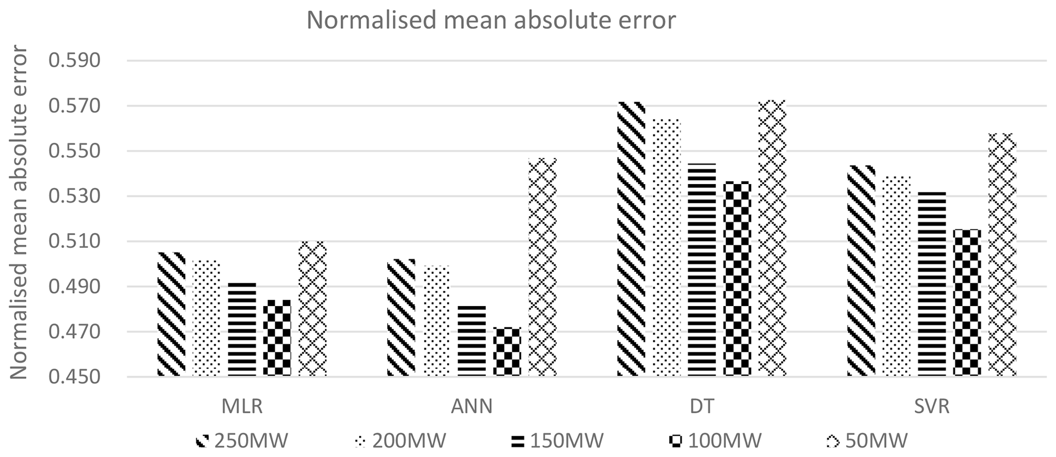
Figure 27 Comparison of the normalised mean absolute error for the various wind farm topologies and MCP methodology, for the 2015 energy output from the wind farm.

The ANN methodology also shows the best similarity to the actual wind speed and wind direction, as seen in Fig. 24. In the case of the overall energy yield, the MLR and ANN methodologies show a significant improvement in percentage error over the DT and SVR methodologies. The ANN methodology is only better than the MLR methodology for the 250 MW wind farm capacity. The MLR methodology has better results in the case of 200, 150, 100 and 50 MW wind farm capacities, with the percentage error being 3.65 % at a wind farm capacity of 50 MW, when compared to an error of 7.3 % obtained with the ANN methodology.

Thus, the metrics show that the best methodology for predicting the output power from the wind farm is therefore MLR, closely followed by ANNs.

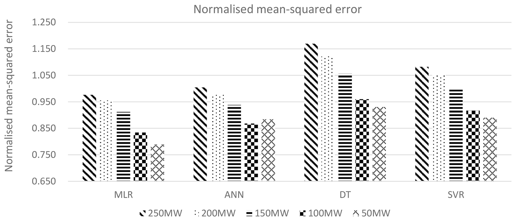
Figure 28 Comparison of the normalised mean-squared error for the various wind farm topologies and MCP methodology, for the 2015 energy output from the wind farm.

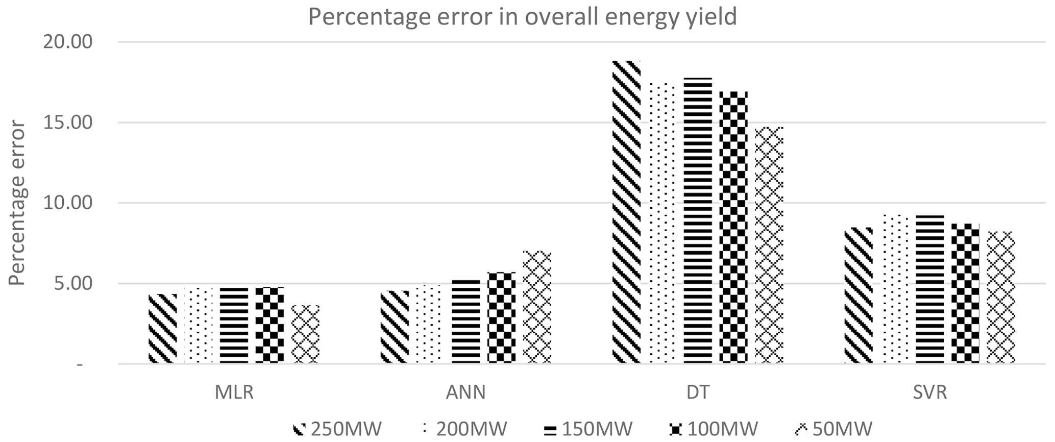
Figure 29 Comparison of the percentage error in overall energy yield for the various wind farm topologies and MCP methodology, for the 2015 energy output from the wind farm.

7 Conclusions

The above research has combined the use of MCP methodologies for wind speed and used a different method for predicting the wind direction at a candidate site. Three of the four MCP methodologies used are based on modern statistical learning methodologies. The data were collected from a reference site which is the island of Malta's international airport, while the candidate site data have been collected by means of a lidar wind measurement system placed on the rooftop of a coastal building.

The wind direction at the candidate site was predicted with the various MCP methodologies by breaking down the wind velocity vector into its respective north and east direction components. The regression analysis was then carried out on the respective components at the reference and the candidate sites. The wind speed is predicted by using the magnitude of the wind speed at the respective sites for creating the regression model. The projected wind speed and direction time series were applied to a hypothetical wind farm. Thus, the error introduced by the four MCP methods could be measured. This was done by calculating the NMAE, the NMSE and the percentage error in the wind farm's energy yield. The results show that the NMAE, NMSE and percentage error in energy yield depend on the MCP methodology and the wind farm capacity and can be used to establish an optimal MCP methodology.

In this case, the best MCP method was that which used MLR. Although other MCP methodologies gave larger errors, they cannot be totally discarded. It is always best to compare methodologies, comparing results by analysing residuals and errors and then choosing the best methodology on a case-by-case basis. In this case the results from the ANN methodology were very close to those of the MLR methodology, while the DT and SVR methodologies gave larger errors.

Unless actual wind data are available, one cannot carry out this analysis, as the uncertainty is obtained by comparing the energy from the wind farm with predicted and actual wind data. The above analysis could be done because 18 months of data were available, rather than the normal 12 months, which is usual for a wind resource assessment which uses MCP methodologies.

The above study was limited to using the same MCP methodology for both the wind speed and the direction and to the N.Ø. Jensen methodology for wake losses. The layout chosen was one that ensured a recommended minimum distance between the wind turbines. Different combinations of MCP methodologies for wind speed and direction can be examined.

In this case, an MCP model was created for wind speed, and two more MCP models were created for wind speed components, which were then used to calculate the wind direction. Another possible method is to calculate the magnitude of the wind speed from the models used to calculate the wind direction. This was done, but the results from the first method were by far superior to those from the latter method. The reason why still needs to be investigated as part of future work is are not presented in this paper. Having three models also allows the possibility of using different combinations of MCP methodologies, i.e. using MLR for wind speed and ANNs for wind direction. This was also performed for a limited number of combinations and is also the subject of further research.

Another area which warrants further study is trying out different wind farm topologies or selecting different wind turbines and different hub heights. It would also be of interest to study the application of different wake methodologies as a possible means of decreasing the uncertainties.

Appendix A: Nomenclature

ANN	Artificial neural network
CFD	Computational fluid dynamics
DTs	Decision trees
Lidar	Light detection and ranging
LES	Large-eddy simulation
MCP	Measure–correlate–predict
MIA	Malta International Airport
MLR	Multiple linear regression
MLP	Multilayer perceptron
MSE	Mean-squared error
NMAE	Normalised mean absolute error
NMSE	Normalised mean-squared error
SLR	Simple linear regression
Sodar	Sonic detection and ranging
SVR	Support vector regression
WT	Wind turbine
Vi	Magnitude of wind speed in metres per second
$e_{{\mathrm{norm}}_i}$	Normalised residual
eeng	Percentage error in energy yield
ei	Residual, MW
${\mathit{u}}_{i_{\mathrm{p}}}$	Predicted component of wind speed vector in the easterly direction at the candidate site in metres per second
${\mathit{u}}_{i_{\mathrm{ref}}}$	Component of wind speed vector in the easterly direction at the reference site in metres per second
${\mathit{u}}_{i_{\mathrm{ref}}}$	Component of wind speed vector in the easterly direction at the reference site in metres per second
ui	Component of wind speed vector in the easterly direction in metres per second
${\mathit{v}}_{i_{\mathrm{can}}}$	Component of wind speed vector in the northerly direction at the candidate site in metres per second
${\mathit{v}}_{i_{\mathrm{p}}}$	Predicted component of wind speed vector in the northerly direction at the candidate site in metres per second
${\mathit{v}}_{i_{\mathrm{ref}}}$	Component of wind speed vector in the northerly direction at the reference site in metres per second
vi	Component of wind speed vector in the northerly direction in metres per second
z0	Surface roughness
Vi	Wind speed vector (speed in metres per second and wind direction in degrees)
${\mathit{\theta }}_{{\mathrm{math}}_{i_{\mathrm{p}}}}$	Predicted mathematical wind direction at the candidate site in degrees
${\mathit{\theta }}_{{\mathrm{met}}_{i_{\mathrm{p}}}}$	Predicted meteorological wind direction at the reference site in degrees
${\mathit{\theta }}_{{\mathrm{met}}_{\mathrm{can}}}$	Meteorological wind direction at the candidate site in degrees
${\mathit{\theta }}_{{\mathrm{met}}_{\mathrm{ref}}}$	Meteorological wind direction at the reference site in degrees
θmath	Mathematical wind direction
θmet	meteorological wind direction
D	Wind turbine diameter, m
N	Number of data points
P	Predicted power output from wind farm, MW
Pact	Actual power output from wind farm, MW